Introduction
In Boltzmann's groundbreaking work, he discovered a fascinating phenomenon known as the "breath mode," where a dilute gas confined in a perfectly isotropic three-dimensional (3D) harmonic potential fails to reach equilibrium and instead exhibits perpetual oscillations in density, velocity, and temperature [1, 2]. This absence of damping in the breath mode posed a challenge to Boltzmann's claim of establishing a microscopic, atomistic foundation for thermodynamics[3]. Due to the absence of experimental confirmation in a three-dimensional system, Boltzmann's prediction regarding the breath mode remained on the periphery of scientific interest for a considerable period. A recent significant study demonstrated the existence of the breath mode in a large collection of Rb cold atoms confined in a harmonic trap, providing strong experimental evidence that aligns with the theoretical predictions [3]. However, M.I. García de Soria et al. [6] have shed other new light on the breath mode, revealing that it is not an eternal solution of the system. Their research shows that an original dissipative mechanism, primarily associated with the often neglected bulk viscosity, is at play. This mechanism eventually leads to the thermalization of the system, challenging the notion of the breath mode as a perpetual oscillation.
In M.I.García de Soria's study, the researchers utilized molecular dynamics simulations to examine the long-term evolution of the system. They observed that, over time, the oscillation period undergoes slight changes. However, molecular dynamics, being a microscopic method, is too computationally expensive when the Knudsen number increases, indicating a large number of atoms and collisions in the system. In such cases, the use of an asymptotic preserving numerical method becomes essential. This numerical approach enables accurate determination of the relaxation time of the system when it reaches final thermodynamic equilibrium and establishes the relationship between the relaxation time and the Knudsen number. By employing such a method, we can obtain precise insights into the dynamics and behavior of the system.
The Unified Gas-Kinetic Wave-Particle (UGKWP) method is a recently developed multiscale approach that exhibits asymptotic preserving capabilities [7]. UGKWP utilizes a finite volume method and uses the solution to the kinetic equation to compute the flux across cell interfaces. The solution is represented partially by particles to capture the non-equilibrium contributions from nonlocal field, and partially by waves to represent the equilibrium part of the local field.In the collisionless regime, UGKWP has been rigorously validated against the Direct Simulation Monte Carlo (DSMC) method, which serves as a benchmark method for rarefied gas simulations. In the strong collisional regime, UGKWP has been compared to hydrodynamic solvers, demonstrating its effectiveness in capturing multiscale phenomena. Besides, UGKWP has been extended to various fields, including photon transport, neutral transport, and plasma transport, consistently delivering accurate results across these diverse applications[8,9,10].
In this study, we employ the Unified Gas-Kinetic Wave-Particle (UGKWP) method to investigate the long-term evolution of the "breath mode" under varying Knudsen numbers. Our primary focus is to examine the relationship between the Knudsen number and the relaxation time of the system.
Model setting
Kinetic model
The Boltzmann equation for single-component monatomic gas with external force is \[ \frac{\partial f}{\partial t}+\boldsymbol{u}\cdot \nabla_x f+\boldsymbol{a}\cdot \nabla_u f= Q(f,f), \\ \]
where \(f = f(t, \boldsymbol{x}, \boldsymbol{u})\) is the velocity distribution function at space and time \((\boldsymbol{x},t)\) and microscopic translational velocity \(\boldsymbol{u}\). \(\boldsymbol{a}\) is the external force. The binary collisions are described by the collision \(Q(f,f)\),
\[ Q(f, f)=\int_{\mathcal{R}^3} \int_{\mathcal{S}^2}\left(f_*^{\prime} f^{\prime}-f_* f\right)\left|\mathbf{u}_{\mathbf{r}}\right| \sigma d \Omega d \mathbf{u}_* \]
Here the short hand notation \(f_*^{\prime}=f\left(\mathbf{x}, t, \mathbf{u}_*^{\prime}\right)\) is used, similarly for \(f^{\prime}\) and \(f_*\), where \(\mathbf{u}\), \(\mathbf{u}_*\) are the pre-collision particle velocities and \(\mathbf{u}^{\prime}, \mathbf{u}_*^{\prime}\) are the corresponding post-collision velocities. \(\Omega\) is a unit vector in \(\mathcal{S}^2\) along the relative post-collision velocity \(\mathbf{u}^{\prime}-\mathbf{u}^{\prime}{ }_*\). The differential cross section \(\sigma\) measures the probability of collision which depends on the strength of relative velocity and deflection angle between pre-collision and post-collision velocities.
In this article, kinetic model equations are proposed to simplify the Boltzmann equation, in which the colision terms are modeled by a relaxation-type BGK operator,
\[ Q\equiv \frac{g-f}{\tau} \]
where \(g\) is the local equilibrium distribution function and \(\tau\) is the relaxtion time. The Maxwellian distribution for 1D problem is
\[ g = \rho\left(\frac{\lambda}{\pi}\right)^{\frac{K+1}{2}}e^{-\lambda((u-U)^2+\xi^2)}, \]
where \(\rho\) is density, \(\lambda=m/2kT\), \(m\) is molecule mass, \(k\) is Boltzmann constant, \(U\) is the macroscopic velocity, \(K\) is the number of internal degree of freedom and \(\xi^2=\xi_1^2+\xi_2^2...+\xi_K^2\). For example, a monatomic gas at 1D problem has \(K=2\) to account for the motion in \(y,z\) direction, and \(\xi^2=v^2+w^2\), where \(v,w\) are particle velocity in \(y,z\) direction.
The relation between \(K\) and the ratio of specific heat is,
\[ \gamma = \frac{K+3}{K+1}. \]
In this article, we calculate 1D problem using 3D framework, so \(K=0\) and \(\gamma=5/3\).
Viscosity model
The dynamic viscosity can be calculated from Sutherland's law or hard-sphere(HS)/variable hard-sphere model(VHS)[11],
\[ \mu = \mu_{ref}\left(\frac{T}{T_{ref}}\right)^\omega, \]
where \(\mu_{ref}\) is the reference viscosity and \(T_{ref}\) is the reference temperature, \(\omega\) is the index related to HS or VHS model. Here we use \(\omega=0.72\). \(T_{ref}=1\) in our nondimensional model. The reference viscosity can be calculated through, \[ \mu_{ref} = \frac{5(\alpha+1)(\alpha+2)\sqrt{\pi}}{4\alpha(5-2\omega)(7-2\omega)}Kn \] where \(\alpha\) is coefficients related to the molecule model. Here we use \(\alpha=1.0\).
The relaxation time can be calculate through the relation
\[ \tau = \frac{\mu}{p} = \frac{1}{p}\left(\frac{T}{T_{ref}}\right)^\omega\frac{5(\alpha+1)(\alpha+2)\sqrt{\pi}}{4\alpha(5-2\omega)(7-2\omega)}Kn \]
In some literature, \(\tau = Kn\) is used as simplified model between relaxation time and Knudsen number, here in our model, we use more collision model.
Potential model
In this article, we employ an electrostatic potential to confine electrons. The ions in the system form a uniform background, resulting in a charge density denoted as \(\rho_0 = n_i e\), where \(n_i\) represents the ion density and \(e\) is the elementary charge. When \(\rho_0 > 0\), a positive potential emerges between the two boundaries.In our work, we consider \(n_i = 1\) and \(e = 1\). By introducing a group of electrons into the domain with zero initial velocity,ignoring collisions and electrons influence on the electric field, the electrons feel harmonic forces and undergo periodic oscillations.
Applying Gauss's law, we find that the Laplacian of the electrostatic potential, denoted as \(\phi\), is given by
\[ \nabla^2 \phi = -\frac{\rho_0}{\epsilon_0} \]
where \(\epsilon_0\) represents the vacuum permittivity. Additionally, the electric field \(\mathbf{E}\) can be expressed as \(\mathbf{E} = -\nabla \phi\).
Explicitly calculating the electric field, we obtain \(E = x\), resulting in the electrons experiencing a force of \(F = -q_eE = -x\), where \(q_e\) represents the charge of an electron. In this study, we assume the electron mass \(m_e\) to be equal to 1. Consequently, the equation of motion for the electrons can be written as
\[ m_e \frac{d^2x}{dt^2} = F\]
which simplifies to \(\frac{d^2x}{dt^2} = -x\). Solving this second-order differential equation yields the solution
\[ x = c_1\cos(t) + c_2\sin(t) = c\sin(t+\phi) \] where \(c_1\) and \(c_2\) depend on the initial conditions.
From the solution, it is evident that the electrons undergo harmonic oscillations with frequency \(\omega=1, T=2\pi\), with the amplitude and phase determined by the constants \(c\) and \(\phi\), respectively.
In the context of a harmonic oscillator, the force acting on the electrons can be expressed as \(F = -m_e\omega^2 x\). Here, we assume that the electron mass, denoted as \(m_e\), is equal to 1, and the angular frequency, represented by \(\omega\), is also equal to 1.
UGKWP method
These papers [7,12] outlines the detailed process of the UGKWP method. In this article, we just add an external force. The general procedure of the algorithm is
- Initalize simulation particles into the domain.
- Update conservative variables \(\mathbf{W}\) to \(\mathbf{W}^{*}\) considering net flux without force term by UGKWP acorss the cell interface.
- Incorporate the interaction between harmonic potential field and particles, and evolve \(\mathbf{W}^{*}\) to \(\mathbf{W}^{n+1}\)
- Run until finish condition.
Here we use the Leap-frog method to realize a second-order accuracy of motion.
Flux in UGKWP
Results
Prieodic ocillation in the collisionless regime
As a verification of code, we first ignore the collision between particles to see whether we can get a periodic osicllation.
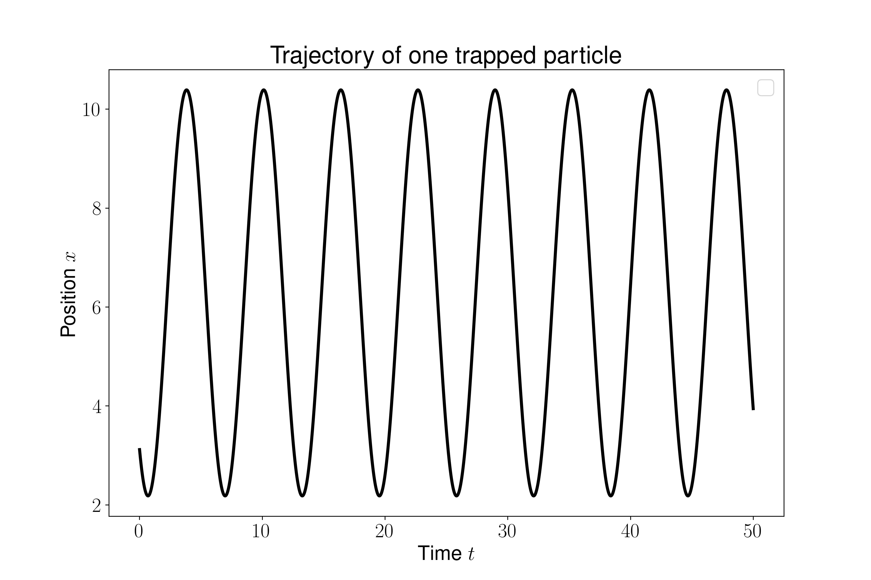
From the figure above we can clearly that the particle in the system oscillate with \(T=2\pi\) without any damping.Here is the video of the density of trapper particles.
Collision regime
For convenience of modeling, here we set \(n_i = 0.01\), so that \(\omega = 0.1\). The domain length is \(4\pi\), and the boundary condition is periodic boundary. The density equilibrium distribution is
\[ n = n_0 e^{-\frac{m\omega^2 r^2}{2k_B T}} = n_0 e^{-\lambda \omega^2 r^2} \]
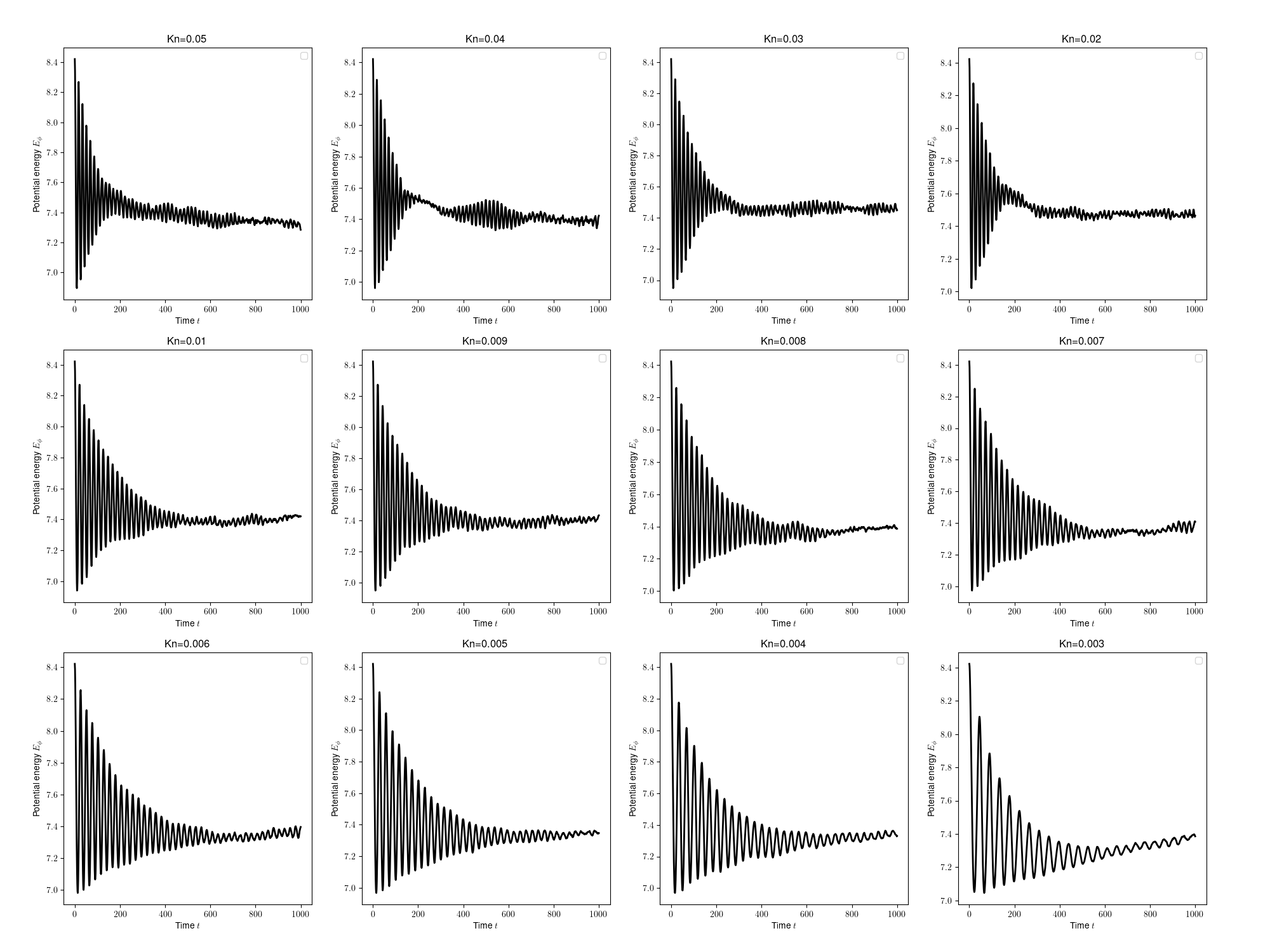
Here \(\lambda = 3/2\). Here the result at \(Kn=0.01\),
For modeling convenience, we set the ion density \(n_i\) to be 0.01, resulting in an angular frequency \(\omega\) of 0.1. The computational domain has a length of \(4\pi\) units, and we impose periodic boundary conditions.
The equilibrium density distribution in the system can be described by the expression \[ n = n_0 e^{-\frac{m\omega^2 r^2}{2k_B T}} \], where \(n_0\) represents the normalized reference density and \(k_B\) is the Boltzmann constant. In this particular case, we have \(\lambda = \frac{3}{2}\), indicating that the density decays exponentially with \(\omega^2 r^2\).
The specific results obtained at a Knudsen number of 0.01 are as follows:
From the image and accompanying video, it is apparent that the system eventually reaches an equilibrium state. Here is the decay of potential energy at multiplie Knudesen numbers.
Analysis
Reference
[1]. F. Hasenöhrl, L. Boltzmann, eds., Über die Aufstellung und Integration der Gleichungen, welche die Molekularbewegung in Gasen bestimmen, in: Wissenschaftliche Abhandlungen, Cambridge University Press, Cambridge, 2012: pp. 55–102. https://doi.org/10.1017/CBO9781139381437.005.
[2]. C. Cercignani, The Boltzmann Equation and Its Applications, Springer, New York, NY, 1988. https://doi.org/10.1007/978-1-4612-1039-9.
[3]. D.S. Lobser, A.E.S. Barentine, E.A. Cornell, H.J. Lewandowski, Observation of a persistent non-equilibrium state in cold atoms, Nature Phys 11 (2015) 1009–1012. https://doi.org/10.1038/nphys3491.
[4] F. Chevy, V. Bretin, P. Rosenbusch, K.W. Madison, J. Dalibard, Transverse Breathing Mode of an Elongated Bose-Einstein Condensate, Phys. Rev. Lett. 88 (2002) 250402. https://doi.org/10.1103/PhysRevLett.88.250402.
[5] T. Kinoshita, T. Wenger, D.S. Weiss, A quantum Newton’s cradle, Nature 440 (2006) 900–903. https://doi.org/10.1038/nature04693.
[6] M.I. García de Soria, P. Maynar, D. Guéry-Odelin, E. Trizac, Fate of Boltzmann’s Breathers: Stokes Hypothesis and Anomalous Thermalization, Phys. Rev. Lett. 132 (2024) 027101. https://doi.org/10.1103/PhysRevLett.132.027101.
[7] C. Liu, Y. Zhu, K. Xu, Unified gas-kinetic wave-particle methods I: Continuum and rarefied gas flow, Journal of Computational Physics 401 (2020) 108977. https://doi.org/10.1016/j.jcp.2019.108977.
[8] W. Li, C. Liu, Y. Zhu, J. Zhang, K. Xu, Unified gas-kinetic wave-particle methods III: Multiscale photon transport, Journal of Computational Physics 408 (2020) 109280. https://doi.org/10.1016/j.jcp.2020.109280.
[9] C. Liu, K. Xu, Unified gas-kinetic wave-particle methods IV: multi-species gas mixture and plasma transport, Advances in Aerodynamics 3 (2021) 9. https://doi.org/10.1186/s42774-021-00062-1.
[10] X. Xu, Y. Chen, C. Liu, Z. Li, K. Xu, Unified gas-kinetic wave-particle methods V: Diatomic molecular flow, Journal of Computational Physics 442 (2021) 110496. https://doi.org/10.1016/j.jcp.2021.110496.
[11] R.Wang, K.Xu, User’s Manual for UGKS1D and UGKS2D Codes
[12] Y.(朱亚军) Zhu, C.(刘畅) Liu, C.(钟诚文) Zhong, K.(徐昆) Xu, Unified gas-kinetic wave-particle methods. II. Multiscale simulation on unstructured mesh, Physics of Fluids 31 (2019) 067105. https://doi.org/10.1063/1.5097645.