Contour integral by Landau
As an elementary illustration of the use of the Vlasov equation, we shall derive the dispersion relation for electron plasma oscillations, which we treated from the fluid point of view in Sect. 4.3. This derivation will require a knowledge of contour integration. Those not familiar with this may skip to Sect. 7.5. A simpler but longer derivation not using the theory of complex variables appears in Sect. 7.6.
In zeroth order, we assume a uniform plasma with a distribution \(f_0(\mathbf{v})\), and we let \(\mathbf{B}_0=\mathbf{E}_0=0\). In first order, we denote the perturbation in \(f(\mathbf{r}, \mathbf{v}, t)\) by \(f_1(\mathbf{r}, \mathbf{v}, t)\) : \[ f(\mathbf{r}, \mathbf{v}, t)=f_0(\mathbf{v})+f_1(\mathbf{r}, \mathbf{v}, t) \]
Since \(\mathbf{v}\) is now an independent variable and is not to be linearized, the first-order Vlasov equation for electrons is \[ \frac{\partial f_1}{\partial t}+\mathbf{v} \cdot \nabla f_1-\frac{e}{m} \mathbf{E}_1 \cdot \frac{\partial f_0}{\partial \mathbf{v}}=0 \]
As before, we assume the ions are massive and fixed and that the waves are plane waves in the \(x\) direction \[ f_1 \propto e^{i(k x-\omega t)} \]
Then Eq. (7.45) becomes \[ \begin{gathered} -i \omega f_1+i k v_x f_1=\frac{e}{m} E_x \frac{\partial f_0}{\partial v_x} \\ f_1=\frac{i e E_x}{m} \frac{\partial f_0 / \partial v_x}{\omega-k v_x} \end{gathered} \]
Poisson's equation gives \[ \varepsilon_0 \boldsymbol{\nabla} \cdot \mathbf{E}_1=i k \varepsilon_0 E_x=-e n_1=-e \iiint f_1 d^3 v \]
Substituting for \(f_1\) and dividing by \(i k \varepsilon_0 E_x\), we have \[ 1=-\frac{e^2}{k m \varepsilon_0} \iiint \frac{\partial f_0 / \partial v_x}{\omega-k v_x} d^3 v \]
A factor \(n_0\) can be factored out if we replace \(f_0\) by a normalized function \(\hat{f}_0\) : \[ 1=-\frac{\omega_p^2}{k} \int_{-\infty}^{\infty} d v_z \int_{-\infty}^{\infty} d v_y \int_{-\infty}^{\infty} \frac{\partial \hat{f}_0\left(v_x, v_y, v_z\right) / \partial v_x}{\omega-k v_x} \partial v_x \]
If \(f_0\) is a Maxwellian or some other factorable distribution, the integrations over \(v_y\) and \(v_z\) can be carried out easily. What remains is the one-dimensional distribution \(\hat{f}_0\left(v_x\right)\). For instance, a one-dimensional Maxwellian distribution is \[ \hat{f}_m\left(v_x\right)=(m / 2 \pi K T)^{1 / 2} \exp \left(-m v_x^2 / 2 K T\right) \]
The dispersion relation is, therefore, \[ 1=\frac{\omega_p^2}{k^2} \int_{-\infty}^{\infty} \frac{\partial \hat{f}_0\left(v_x\right) / \partial v_x}{v_x-(\omega / k)} \] (这是一个积分区间在实轴,但是被积函数是复变函数的例子,这个时候应该将积分延拓到复数区间,然后想办法消去复数部分的积分,详见梁昆淼《数学物理方法》4.2节。) Since we are dealing with a one-dimensional problem we may drop the subscript \(x\), being careful not to confuse \(v\) (which is really \(v_x\) ) with the total velocity \(v\) used earlier: \[ 1=\frac{\omega_p^2}{k^2} \int_{-\infty}^{\infty} \frac{\partial \hat{f}_0 / \partial v}{v-(\omega / k)} d v \]
Here, \(\hat{f}_0\) is understood to be a one-dimensional distribution function, the integrations over \(v_y\) and \(v_z\) having been made. Equation (7.54) holds for any equilibrium distribution \(\hat{f}_0(v)\); in particular, if \(\hat{f}_0\) is Maxwellian, Eq. (7.52) is to be used for it.
The integral in Eq. (7.54) is not straightforward to evaluate because of the singularity at \(v=\omega / k\). One might think that the singularity would be of no concern, because in practice \(\omega\) is almost never real; waves are usually slightly damped by collisions or are amplified by some instability mechanism. Since the velocity \(v\) is a real quantity, the denominator in Eq. (7.54) never vanishes. Landau was the first to treat this equation properly. He found that even though the singularity lies off the path of integration, its presence introduces an important modification to the plasma wave dispersion relation - an effect not predicted by the fluid theory.
Consider an initial value problem in which the plasma is given a sinusoidal perturbation, and therefore \(k\) is real. If the perturbation grows or decays, \(\omega\) will be complex. The integral in Eq. (7.54) must be treated as a contour integral in the complex \(v\) plane. Possible contours are shown in Fig. 7.14 for (a) an unstable wave, with \(\operatorname{Im}(\omega)>0\), and (b) a damped wave, with \(\operatorname{Im}(\omega)<0\). Normally, one would evaluate the line integral along the real \(v\) axis by the residue theorem: \[ \int_{C_1} G d v+\int_{C_2} G d v=2 \pi i R(\omega / k) \]
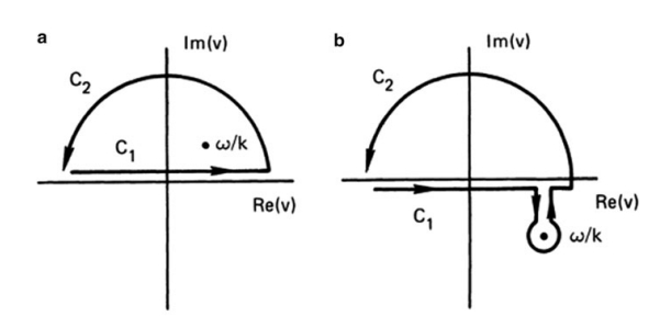
where \(G\) is the integrand, \(C_1\) is the path along the real axis, \(C_2\) is the semicircle at infinity, and \(R(\omega / k)\) is the residue at \(\omega / k\). This works if the integral over \(C_2\) vanishes.(如果C2的路径积分可以消失,那么就可以比较方便的得出实轴上的积分,但是很可惜,在Maxwell分布的前提下,虚部积分不能消去,这个时候Landau提出了另一种积分方法,详见Cairns的推导。按照Landau的方法,积分路径就不包含类似于C2的部分,只存在实轴的积分以及有限个靠近实轴的奇点,用留数定理就可以求解。) Unfortunately, this does not happen for a Maxwellian distribution, which contains the factor \[ \exp \left(-v^2 / v_{\mathrm{th}}^2\right) \]
This factor becomes large for \(v \rightarrow \pm i \infty\), and the contribution from \(C_2\) cannot be neglected. Landau showed that when the problem is properly treated as an initial value problem the correct contour to use is the curve \(C_1\) passing below the singularity. This integral must in general be evaluated numerically, and Fried and Conte have provided tables for the case when \(\hat{f}_0\) is a Maxwellian.
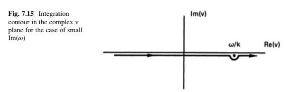
Although an exact analysis of this problem is complicated, we can obtain an approximate dispersion relation for the case of large phase velocity and weak damping. In this case, the pole at \(\omega / k\) lies near the real \(v\) axis (Fig. 7.15). The contour prescribed by Landau is then a straight line along the \(\operatorname{Re}(v)\) axis with a small semicircle around the pole. In going around the pole, one obtains \(2 \pi i\) times half the residue there. Then Eq. (7.54) becomes \[ 1=\frac{\omega_p^2}{k^2}\left[P \int_{-\infty}^{\infty} \frac{\partial \hat{f}_0 / \partial v}{v-(\omega / k)} d v+\left.i \pi \frac{\partial \hat{f}_0}{\partial v}\right|_{v=\omega / k}\right] \]
此处,\(Res(f(z_0)) = \frac{P(z_0)}{Q^{'}(z_0)} = \frac{\partial \hat{f}_0 / \partial v}{(v-(\omega / k))^{'}}|_{v=v_{\phi}} = \frac{\partial \hat{f}_0 }{\partial v}|_{v=v_{\phi}}\), 参考梁昆淼p53.
where \(P\) stands for the Cauchy principal value. To evaluate this, we integrate along the real \(v\) axis but stop just before encountering the pole. If the phase velocity \(v_\phi=\omega / k\) is sufficiently large, as we assume, there will not be much contribution from the neglected part of the contour, since both \(\hat{f}_0\) and \(\partial \hat{f}_0 / \partial v\) are very small there (Fig. 7.16). The integral in Eq. (7.56) can be evaluated by integration by parts: \[ \int_{-\infty}^{\infty} \frac{\partial \hat{f}_0}{\partial v} \frac{d v}{v-v_\phi}=\left[\frac{\hat{f}_0}{v-v_\phi}\right]_{-\infty}^{\infty}-\int_{-\infty}^{\infty} \frac{-\hat{f}_0 d v}{\left(v-v_\phi\right)^2}=\int_{-\infty}^{\infty} \frac{\hat{f}_0 d v}{\left(v-v_\phi\right)^2} \]
Since this is just an average of \(\left(v-v_\phi\right)^{-2}\) over the distribution, the real part of the dispersion relation can be written \[ 1=\frac{\omega_p^2}{k^2} \overline{\left(v-v_\phi\right)^{-2}} \]
Since \(v_\phi \gg v\) has been assumed, we can expand \(\left(v-v_\phi\right)^{-2}\) : \[ \left(v-v_\phi\right)^{-2}=v_\phi^{-2}\left(1-\frac{v}{v_\phi}\right)^{-2}=v_\phi^{-2}\left(1+\frac{2 v}{v_\phi}+\frac{3 v^2}{v_\phi^2}+\frac{4 v^3}{v_\phi^3}+\cdots\right) \]
The odd terms vanish upon taking the average, and we have \[ \overline{\left(v-v_\phi\right)^{-2}} \approx v_\phi^{-2}\left(1+\frac{3 \overline{v^2}}{v_\phi^2}\right) \]
We now let \(\hat{f}_0\) be Maxwellian and evaluate \(\overline{v^2}\). Remembering that \(v\) here is an abbreviation for \(v_x\), we can write \[ \frac{1}{2} m \overline{v_x^2}=\frac{1}{2} K T_e \] there being only one degree of freedom. The dispersion relation (7.58) then becomes \[ \begin{gathered} 1=\frac{\omega_p^2}{k^2} \frac{k^2}{\omega^2}\left(1+3 \frac{k^2}{\omega^2} \frac{K T_e}{m}\right) \\ \omega^2=\omega_p^2+\frac{\omega_p^2}{\omega^2} \frac{3 K T_e}{m} k^2 \end{gathered} \]
If the thermal correction is small(recall 在冷等离子体中\(\omega=\omega_p\), 不存在\(k\), 这就是这里不考虑热修正的意思), we may replace \(\omega^2\) by \(\omega_p^2\) in the second term. We then have \[ \omega^2=\omega_p^2+\frac{3 K T_e}{m} k^2 \] which is the same as Eq. (4.30), obtained from the fluid equations with \(\gamma=3\). We now return to the imaginary term in Eq. (7.56). In evaluating this small term, it will be sufficiently accurate to neglect the thermal correction to the real part of \(\omega\) and let \(\omega^2 \approx \omega_p^2\). From Eqs. (7.57) and (7.60), we see that the principal value of the integral in Eq. (7.56) is approximately \(k^2 / \omega^2\). Equation (7.56) now becomes \[ \begin{gathered} 1=\frac{\omega_p^2}{\omega^2}+\left.i \pi \frac{\omega_p^2}{k^2} \frac{\partial \hat{f}_0}{\partial v}\right|_{v=v_\phi} \\ \omega^2\left(1-i \pi \frac{\omega_p^2}{k^2}\left[\frac{\partial \hat{f}_0}{\partial v}\right]_{v=v_\phi}\right)=\omega_p^2 \end{gathered} \]
Treating the imaginary term as small, we can bring it to the right-hand side and take the square root by Taylor series expansion. We then obtain \[ \omega=\omega_p\left(1+i \frac{\pi}{2} \frac{\omega_p^2}{k^2}\left[\frac{\partial \hat{f}_0}{\partial v}\right]_{v=v_\phi}\right) \]
If \(\hat{f}_0\) is a one-dimensional Maxwellian, we have \[ \frac{\partial \hat{f}_0}{\partial v}=\left(\pi v_{\mathrm{th}}^2\right)^{-1 / 2}\left(\frac{-2 v}{v_{\mathrm{th}}^2}\right) \exp \left(\frac{-v^2}{v_{\mathrm{th}}^2}\right)=-\frac{2 v}{\sqrt{\pi} v_{\mathrm{th}}^3} \exp \left(\frac{-v^2}{v_{\mathrm{th}}^2}\right) \]
We may approximate \(v_\phi\) by \(\omega_p / k\) in the coefficient, but in the exponent we must keep the thermal correction in Eq. (7.64). The damping is then given by \[ \begin{aligned} \operatorname{Im}(\omega) & =-\frac{\pi}{2} \frac{\omega_p^3}{k^2} \frac{2 \omega_p}{k \sqrt{\pi}} \frac{1}{v_{\mathrm{th}}^3} \exp \left(\frac{-\omega^2}{k^2 v_{\mathrm{th}}^2}\right) \\ & =-\sqrt{\pi} \omega_p\left(\frac{\omega_p}{k v_{\mathrm{th}}}\right)^3 \exp \left(\frac{-\omega_p^2}{k^2 v_{\mathrm{th}}^2}\right) \exp \left(\frac{-3}{2}\right) \\ \operatorname{Im}\left(\frac{\omega}{\omega_p}\right) & =-0.22 \sqrt{\pi}\left(\frac{\omega_p}{k v_{\mathrm{th}}}\right)^3 \exp \left(\frac{-1}{2 k^2 \lambda_{\mathrm{D}}^2}\right) \end{aligned} \]
Since \(\operatorname{Im}(\omega)\) is negative, there is a collisionless damping of plasma waves; this is called Landau damping. As is evident from Eq. (7.70), this damping is extremely small for small \(k \lambda_{\mathrm{D}}\), but becomes important for \(k \lambda_{\mathrm{D}}=O(1)\). This effect is connected with \(f_1\), the distortion of the distribution function caused by the wave.
The meaning of Landau Damping
The theoretical discovery of wave damping without energy dissipation by collisions is perhaps the most astounding result of plasma physics research. That this is a real effect has been demonstrated in the laboratory. Although a simple physical explanation for this damping is now available, it is a triumph of applied mathematics that this unexpected effect was first discovered purely mathematically in the course of a careful analysis of a contour integral. Landau damping is a characteristic of collisionless plasmas, but it may also have application in other fields. For instance, in the kinetic treatment of galaxy formation, stars can be considered as atoms of a plasma interacting via gravitational rather than electromagnetic forces. Instabilities of the gas of stars can cause spiral arms to form, but this process is limited by Landau damping.
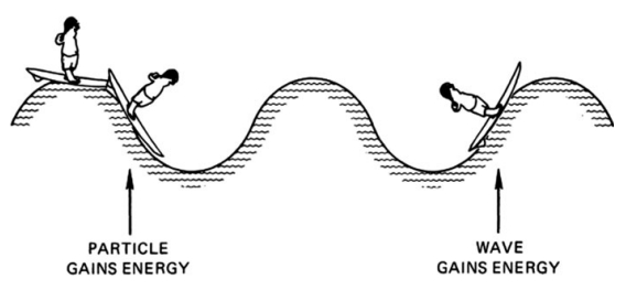
To see what is responsible for Landau damping, we first notice that \(\operatorname{Im}(\omega)\) arises from the pole at \(v=v_\phi\)(因为看色散关系可以看到,在奇点处,由留数贡献的虚部才比较显著). Consequently, the effect is connected with those particles in the distribution that have a velocity nearly equal to the phase velocity - the "resonant particles." These particles travel along with the wave and do not see a rapidly fluctuating electric field: They can, therefore, exchange energy with the wave effectively. The easiest way to understand this exchange of energy is to picture a surfer trying to catch an ocean wave (Fig. 7.17). (Warning: this picture is only for directing our thinking along the right lines; it does not correctly explain Eq. (7.70).) If the surfboard is not moving, it merely bobs up and down as the wave goes by and does not gain any energy on the average. Similarly, a boat propelled much faster than the wave cannot exchange much energy with the wave. However, if the surfboard has almost the same velocity as the wave, it can be caught and pushed along by the wave; this is, after all, the main purpose of the exercise. In that case, the surfboard gains energy, and therefore the wave must lose energy and is damped. On the other hand, if the surfboard should be moving slightly faster than the wave, it would push on the wave as it moves uphill; then the wave could gain energy. In a
plasma, there are electrons both faster and slower than the wave. A Maxwellian distribution, however, has more slow electrons than fast ones (Fig. 7.18). Consequently, there are more particles taking energy from the wave than vice versa, and the wave is damped. As particles with \(v \approx v_\phi\) are trapped in the wave, \(f(v)\) is flattened near the phase velocity. This distortion is \(f_1(v)\) which we calculated. As seen in Fig. 7.18, the perturbed distribution function contains the same number of particles but has gained total energy (at the expense of the wave).
From this discussion, one can surmise that if \(f_0(v)\) contained more fast particles than slow particles, a wave can be excited. Indeed, from Eq. (7.67), it is apparent that \(\operatorname{Im}(\omega)\) is positive if \(\partial \hat{f}_0 / \partial v\) is positive at \(v=v_\phi\). Such a distribution is shown in Fig. 7.19. Waves with \(v_\phi\) in the region of positive slope will be unstable, gaining energy at the expense of the particles. This is just the finite-temperature analogy of the two-stream instability. When there are two cold \((K T=0)\) electron streams in motion, \(f_0(v)\) consists of two \(\delta\)-functions. This is clearly unstable because \(\partial f_0 / \partial v\) is infinite; and, indeed, we found the instability from fluid theory. When the streams have finite temperature, kinetic theory tells us that the relative densities and temperatures of the two streams must be such as to have a region of positive \(\partial f_0 /\) \(\partial v\) between them; more precisely, the total distribution function must have a minimum for instability.
The physical picture of a surfer catching waves is very appealing, but it is not precise enough to give us a real understanding of Landau damping. There are actually two kinds of Landau damping: linear Landau damping, and nonlinear Landau damping. Both kinds are independent of dissipative collisional mechanisms. If a particle is caught in the potential well of a wave, the phenomenon is called "trapping." As in the case of the surfer, particles can indeed gain or lose energy in trapping. However, trapping does not lie within the purview of the linear theory. That this is true can be seen from the equation of motion \[ m d^2 x / d t^2=q E(x) \]
If one evaluates \(E(x)\) by inserting the exact value of \(x\), the equation would be nonlinear, since \(E(x)\) is something like \(\sin k x\). What is done in linear theory is to use for \(x\) the unperturbed orbit; i.e., \(x=x_0+v_0 t\). Then Eq. (7.71) is linear. This approximation, however, is no longer valid when a particle is trapped. When it encounters a potential hill large enough to reflect it, its velocity and position are, of course, greatly affected by the wave and are not close to their unperturbed values. In fluid theory, the equation of motion is \[ m\left[\frac{\partial \mathbf{v}}{\partial t}+(\mathbf{v} \cdot \nabla) \mathbf{v}\right]=q \mathbf{E}(x) \]
Here, \(\mathbf{E}(x)\) is to be evaluated in the laboratory frame, which is easy; but to make up for it, there is the \((\mathbf{v} \cdot \nabla) \mathbf{v}\) term. The neglect of \(\left(\mathbf{v}_1 \cdot \nabla\right) \mathbf{v}_1\) in linear theory amounts to the same thing as using unperturbed orbits. In kinetic theory, the nonlinear term that is neglected is, from Eq. (7.45), \[ \frac{q}{m} E_1 \frac{\partial f_1}{\partial v} \]
When particles are trapped, they reverse their direction of travel relative to the wave, so the distribution function \(f(v)\) is greatly disturbed near \(v=\omega / k\). This means that \(\partial f_1 / \partial v\) is comparable to \(\partial f_0 / \partial v\), and the term (7.73) is not negligible. Hence, trapping is not in the linear theory.
When a wave grows to a large amplitude, collisionless damping with trapping does occur. One then finds that the wave does not decay monotonically; rather, the amplitude fluctuates during the decay as the trapped particles bounce back and forth in the potential wells. This is nonlinear Landau damping. Since the result of Eq. (7.67) was derived from a linear theory, it must arise from a different physical effect. The question is: Can untrapped electrons moving close to the phase velocity of the wave exchange energy with the wave? Before giving the answer, let us examine the energy of such electrons.