Introduction
Solar-Terrestrial physics is principally concerned with the interaction of energetic charged particles with the electic and magnetic fields in space. In the vicinity of the earth, most of these charged particles derive their energy ultimately from the sun or from the interaction of the solar wind with the earth's magnetosphere. These interactions are complex, because the magnetic and electric fields that determine the motion of the particles are affected in turn by the motion of these charged particles. Some solar-terrestrial research is carried out on the surface of the earth with cameras, photometers and spectrometers, and magnetometers and other devices sensitive to the processes occuring high in the upper atmosphere and magnetosphere, but today most of this research is carried out using rockets and satellites that enable measurements to be obtained directly in the regions of strongest interactions. In recent years, these in situ data have resulted in explosive growth in our knowledge and understanding of solar-terrestrial processes. Nevertheless, the field has had a long history of investigation, starting well before the advent of satellites and rockets. We shall briefly review that history in order to provide a context for our later, more physically oriented presentation of the processes occuring in the solar terrestrial environment.
Ancient auroral sightings
The emerging field of solar-terrestrial physics began with a growing appreciation of two phenomena: the aurora and, later, the geomagnetic field. Because it can be observed visually, the aurora was the first of these phenomena to be recorded. Most other phenomena of this emerging field awaited the advent of new technology, such as the compass in the case of geomagnetism, before they were discovered. References to the aurora are contained in the ancient literature from both East and West. Several passages in the Old Testament appear to ahve been inspired by auroral sightings, and Greek literature includes references to phenomena most likely to have been auroral phenomena. For example, Xenophanes, in the sixth centry B.C., mentions "moving accumulations of burning clouds." Chinese literature also describes possible auroral sightings, of which several occured prior to 2000 B.C.
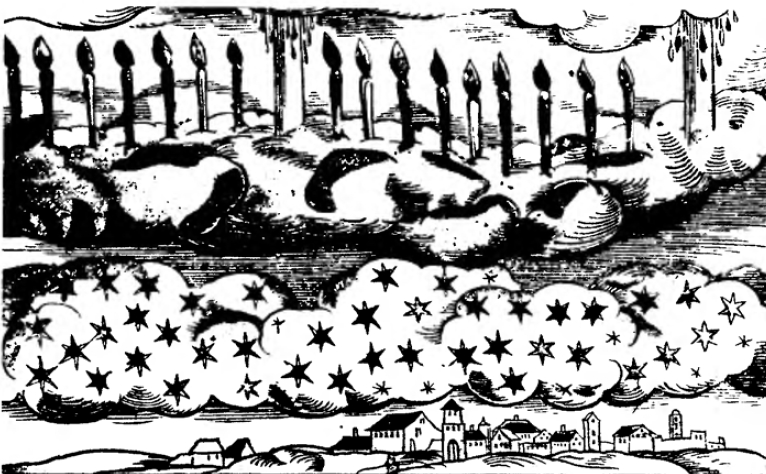
Because the phenomenon was not understood, much fear and superstition surrounded those early sightings of the aurora. The above figure illustrates the lack of scientific understanding of prevalent at that time. The seventeenth century marked the beginning of scientific theories concerning the origin of the lights in the north. Galileo Galilei, for example, proposed that the aurora was caused by air rising out of the earth's shadow to where it could be illuminated by sunlight. He also appears to have coined the term aurora borealis, meaning "dawn of the north." Pierre Gassendi, a French mathematician and astronomer, at about the same time, deduced that auroral displays must be occurring at great heights, because they were seen to have the same configuration when observed at places quite remote from one another. His contemporary, René Descartes, seems to have been the originator of the idea that auroras were caused by reflections from ice crystals in the air at high latitudes. From about 1645 to about 1715, both solar activity and auroral sightings declined, although neither were completely lacking.
Edmund Halley, after finally, at the age of 60, having personally observed an auroral display, seems to have been the first to suggest that the auroral phenomenon was ordered by the direction of the earth's magnetic field. In 1731, the French philosopher de Mairan ridiculed the currently popular idea that the aurora was a reflection of polar ice and snow, and he also criticized Halley's theory. He suggested that the aurora was connected to the solar atmosphere, and he suspected a connection between the return of sunspots and the aurora. After that time, studies of geomagnetism and the aurora became more firmly linked.
Early measurements of the geomagnetic field
The earliest indication of the existence of the geomagnetic field was the direction-finding capability of the compass. As compasses were improved, more and more was learned about the geomagnetic field. The earliest reliable evidence of Chinese knowledge that a compass points north or south dates from the eleventh century. The encyclopedist Shon-Kau (A.D. 1030-93) stated that "fortune-tellers rub the point of a needle with the stone of the magnet in order to make it properly indicate the south.* In the European literature, the earliest mention of the compass and its application to navigation appeared in two works by Alexander Neekan, a monk of St. Albans (A.D. 1157-217), entitled De Untensilibus and De Rerum. In the former he described the use of the magnetic needle to indicate north and noted that mariners used that means to find their course when the sky was cloudy. In the second, he described the needle as being placed on a pivot, a second-generation form of the compass. In neither work did he describe the instrument as a novelty; it was in common use at that time. Official records indicate that by the fourteenth century, many sailing ships carried compasses.
The direction of magnetic north and that of geographic or true north differ over most of the globe. The measure of this difference is called the declination. It is not clear when magnetic declination was actually discovered. However, a letter written by Georg Hartmann, vicar of St. Sebald's at Nürnberg, to Duke Albrecht of Prussia in 1544 showed that he had observed the declination of Rome in 1510 to be 6° east, whereas it was 10° at Nürnberg. Also, it is known that between the years 1538 and 1541, João de Castro made 43 determinations of declination during a voyage along the west coast of India and in the Red Sea.
Perhaps even more im-portant, on April 5, 1741, Hiorter discovered that geomagnetic and auroral activities were correlated. Simultaneous observations in London by Graham confirmed the occurrence of strong geomagnetic activity on that day. In 1770, J. C. Wilcke noted that auroral rays extend upward along the direction of the magnetic field. That was the same year that Captain James Cook first reported the southern counterpart of the aurora borealis, the aurora australis, or "dawn of the south." Twenty years later, the English scientist Henry Cavendish used triangulation to estimate the height of auroras as between 52 and 71 miles. Earlier attempts at triangulation by Halley and Mairan had been much less accurate.
The great advance of the early nineteenth century was the develop ment of a network to make frequent simultaneous observations with widely spaced magnetometers. C. F. Gauss was one of the leaders o that effort and one of the foremost pioneers in the mathematical analysis of the resulting measurements, which allowed contributions to the geo magnetic field from below the surface of the earth to be separated from those contributions arising high in the atmosphere. Meanwhile, Heinrich Schwabe, on the basis of his sunspot measurements taken between 1825 and 1850, deduced that the variation in the number of sunspots was periodic, with a period of about 10 yr. Magnetic observatories had spread to the British colonies by 1839. Edward Sabine was assigned to supervise four of those observatories (Toronto, St. Helena, Cape of Good Hope, and Hobarton). Using the data from those observatories, he was able to show in 1851 that the intensity of geomagnetic disturbances varied in concert with the sunspot cycle.
The next discovery to provide a link between the sun and geomagnetic activity was Richard Carrington's sighting of a great flare of white light on the sun, on September 1, 1859. Carrington, who was sketching sunspot groups at the time, was startled by the flare, and by the time he was able to summon someone to witness the event a minute later, he was dismayed to find that it had weakened greatly in intensity. Fortu-nately, it had been simultaneously noted by another observer some miles away. Furthermore, at the moment of the flare, the Kew Observatory (London) measurements of the magnetic field had been disturbed. Today we realize that that disturbance of the magnetic field was caused by an increase in the electric currents flowing overhead in the earth's iono-sphere. Such currents flow in response to electric fields in the iono-sphere. The extreme radiation by ultraviolet rays and x-rays from the flare increased the ionization and hence the electrical conductivity of the ionosphere, causing more current to flow in response to the unaltered electric field. Finally, 18 h later, one of the strongest magnetic storms ever recorded broke out. Auroras were seen as far south as Puerto Rico.
To have arrived that quickly, the disturbance would have had to travel from the sun at over 2,300 \(km\cdot s^{-1}\), but \(2,300 km\cdot s^{-1}\) is a high velocity even for the disturbed solar wind. When such disturbances arrive at the earth, the terrestrial field jumps quite abruptly, indicating that the discontinuity in the interplanetary medium that is flowing by the earth is quite thin. The thinness of these disturbance fronts strongly suggests that they are caused by shocks in the interplanetary medium, despite the collisionless nature of the gas there. Usually, collisions are needed to account for the dissipation and heating that occur at a shock. That was the first indication of the existence of collisionless shocks, which since the advent of interplanetary exploration have been found to be ubiquitous in the solar system. Shortly after those observations, in 1861, Balfour Stewart noted the occurrence of pulsations in the earth's magnetic field, with periods of minutes. We now know that the magnetosphere pulsates at a wide variety of periods.
Precursors to our modern understanding of the aurora began to appear in the late nineteenth century. About 1878, H. Becquerel suggested that particles were shot off from the sun and were guided by the earth's magnetic field to the auroral zone. He believed that sunspots ejected protons. A similar theory was espoused by E. Goldstein. In 1897, the great Norwegian physicist Kristian Birkeland made his first auroral expedition to northern Norway. However, it was not until after his third expedition in 1902-3, during which he obtained extensive data on the magnetic perturbations associated with auroras, that he concluded that large electric currents flowed along magnetic-field lines during aurora.
The invention of the vacuum tube led to the understanding that the aurora was in some way similar to the cathode rays in those devices. Soon Sir William Crookes demonstrated that cathode rays were bent by magnetic fields, and shortly thereafter J. J. Thomson showed that cathode rays consisted of the tiny, negatively charged particles we now call electrons. Birkeland adopted those ideas for his auroral theories and attempted to verify his theories with both field observations and laboratory experiments. Specifically, he conducted experiments with a magnetic dipole inside a model earth, which he called a terrella. Those experiments showed that electrons incident on the terrella would produce patterns quite reminiscent of the auroral zone.
K. Birkeland's work inspired the Norwegian mathematician Carl Stormer, whose subsequent calculations of the motion of charged particles in a dipole magnetic field in turn supported Birkeland. As is evident from this photograph, the advent of the camera was an important advance in the study of the aurora. It was through measurements such as these that Stormer accurately determined the height of the aurora.
The ionosphere and magnetosphere
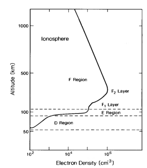
The electrically conducting region above about 100 km altitude that we now call the ionosphere may rightly be claimed to have been discovered by Balfour Stewart. In his 1882 Encyclopaedia Britannica article entitled "Terrestrial Magnetism" he concluded that the upper atmosphere was the most probable location of the electric currents that produce the solar-controlled variation in the magnetic field measured at the surface of the earth. He noted that "we know from our study of aurora that there are such currents in these regions - continuous near the poles and occasional in lower latitudes." He proposed that the primary causes of the daily variations in the intensity of the surface magnetic field were "convective currents established by the sun's heating influence in the upper regions of the atmosphere." These currents "are to be regarded as conductors moving across lines of magnetic force and are thus the vehicle of electric currents which act upon the magnetic field." Those statements are very close to modern atmospheric-dynamo theory. How-ever, it was left to A. Schuster to put the dynamo theory into quantitative form.
The turn of the century brought another new invention that was used to probe the solar-terrestrial environment: the radio transmitter and receiver. In 1902, A.E. Kennelly and O. Heaviside independently postulated the existence of a highly electrically conducting ionosphere to explain G. Marconi's transatlantic radio transmissions. Verification of the existence of the ionosphere did not come until much later, in 1925, when E.V.Appleton and M.A.F. Barnett in the UK, and shortly thereafter G.Breit and M.A. Tuve in America, established the existence and altitude of the Kennelly-Heaviside layer, as it was known hen. The original method of Breit and Tuve, using short pulses of radio energy at vertical incidence and timing the arrival of a reflected signal in order to infer the altitude of the electrically reflecting layer, is still used today for sounding the ionosphere. In drawing diagrams of the electromagnetic waves reflected by the ionosphere, ppleton used the letter E for the electric vector of the downcoming wave. When he found reflections from a higher layer, he used letter F for the electric vector of those reflected waves, and when he occasionally got reflections from a lower layer, he naturally used the letter D. When it came time to name these layers, he chose the same letters, leaving the letters A,B and C for possible later discoveries that never came. So now the ionospheric layers are called the D,E,a nd F layers. We now know that all planets with atmospheres have electrically conducting ionospheres like that of the earth.
At about that same time, progress was being made in understanding the auroral glows. Spectroscopy, together with photography, permitted first the determination of the wavelength and then the identity of the excited molecule that was radiating. There were initial successes, beginning with Lars Vegard's work in Norway relating auroral emissions to emission bands from known atmospheric gases such as nitrogen. However, identification of the yellow-green line at 557.7 nm was elusive.
Finally, H. Babcock's precise measurements in 1923 allowed John McLennan to identify it as a metastable transition of atomic oxygen. At atmospheric pressures close to that at the surface of the earth, collisions between molecules de-excite the molecules before they have a chance to radiate if they happen to become excited into one of the metastable states. However, at the altitude of the aurora, collisions are so rare that the time between collisions is longer than the lifetimes of the metastable states, and the excitation energy of the state can be released by radia-tion. A similar line in the auroral spectrum is the 630.0-m red line of atomic oxygen. This metastable transition has a lifetime of 110s and can radiate only above some 250 km. Those discoveries led to the realization that the varied colors of the aurora were simply related to height.(按:因为不同高度,平均自由程不同,则碰撞频率不同,则会发生不同的辐射。对于碰撞强的地方,metastable的辐射在发生之前就被collision de-excite了,所以不会发生) In low-altitude auroras, below 100 km, where collisions quench even the oxygen green line, the blue and red nitrogen bands predominate. From 100 to 250 km, the oxygen green line is strongest. Above 250 km, the red line is most important.
Although most of the auroral forms are associated with electrons, some aurora are due to precipitating protons. The first observations of the proton aurora were made in 1939. Measurements of the Doppler shifts of the proton emissions permitted estimates of the energy of the precipitating particles from the ground.
With the concept of the ionosphere firmly established, scientists began to wonder about the upper extension of the ionosphere, linked magnetically to the earth, which region we today call the magnetosphere. In 1918, Sydney Chapman postulated a singly-charged beam from the sun as the cause of worldwide magnetic disturbances. That was a revival of an old idea that had previously been criticized by Schuster.Chapman was soon challenged by Frederick Lindemann, who pointed out that mutual electrostatic repulsion would destroy such a stream. Lindemann, instead, suggested that the stream of charged particles contained particles of both signs in equal numbers. We would now call such a stream a "plasma." That proposal was a breakthrough, and it permitted Chapman and his co-workers, in a series of papers beginning in 1930, to lay the foundations for our modern understanding of the interaction of the solar wind with the magnetosphere.
In the rarefied conditions of outer space, where collisions between particles are infrequent, the ion-electron gas, or plasma, is highly electrically conducting. Thus, Chapman and Ferraro proposed that as the plasma from the sun approached the earth, the earth would effectively see a mirror magnetic-dipole moment advancing on the earth. The net result of that advancing mirror field would be to compress the terrestrial field. Eventually, the plasma would surround the earth on all sides, and a cavity would be carved out of the solar plasma by the terrestrial magnetic field. That is very similar to our modern concept of the geomagnetic cavity.
After the compression of the magnetosphere, which is detected by ground-based magnetometers as a sharp increase in the magnetic field, the magnetosphere becomes inflated. Chapman and Ferraro correctly interpreted that subsequent decrease in the magnetic field at the surface of the earth as the appearance of energetic plasma deep inside the magnetosphere, forming a ring of current around the earth in the near-equatorial regions. The development of this ring current in what we now call a geomagnetic storm is discussed at greater length later.
At the same time that the ionosphere was being discovered by virtue of its effects on man-made radio signals, natural radio emissions were also being explored, and the magneto-jonic theory developed for the man-made signals was being applied to those natural emissions. The first report of those electromagnetic signals in the audio-frequency range was an observation of what have become known as "whistlers,"(当时一直有这种噪声干扰无线电波通讯) coming from a 22-km telephone line in Austria in 1886. Whistlers are short bursts of audio-frequency radio noise of continuously decreasing pitch. In 1894, British telephone operators heard "weeks," possibly whistlers generated by lightning, and a "dawn chorus" generated deep in the magnetosphere during a display of aurora borealis. Little work was done on those observations because of the lack of suitable analysis equipment at the time. During World War I, equipment installed to eavesdrop on enemy telephone conversations picked up whistling sounds. Soldiers at the front would say, "You could hear the grenades fly." H. Barkhausen reported on those observations in 1919 and suggested that they were correlated with meteorological influences. However, he could not duplicate the phenomenon in laboratory experiments. In 1925, T. L. Ecker-sley also described that phenomenon and ascribed it to the dispersion of an electrical impulse in a medium loaded with free ions. Eventually, after much work and several incorrect explanations, in 1935 Eckersley concluded that the distinctive swooping sound of whistlers was due to the dispersion of a burst of electromagnetic noise traveling through the ionosphere. Very little work was done on whistlers until the early 1950s, at which time L. R. O. Storey, with a homemade spectrum analyzer, conducted a thorough study of whistlers. He found that whistlers are caused by lightning flashes, whose electromagnetic energy then echoes back and forth along field lines in the upper ionosphere, as illustrated in Figure 1.10. A major implication of those findings was that the electron density in the outer ionosphere, which is now called the plasmasphere, was unexpectedly high. Storey also found other types of audio-frequency, or very low frequency (VLF), emissions that are not associated with lightning and are now known to be generated within the magnetospheric plasma.
The solar wind
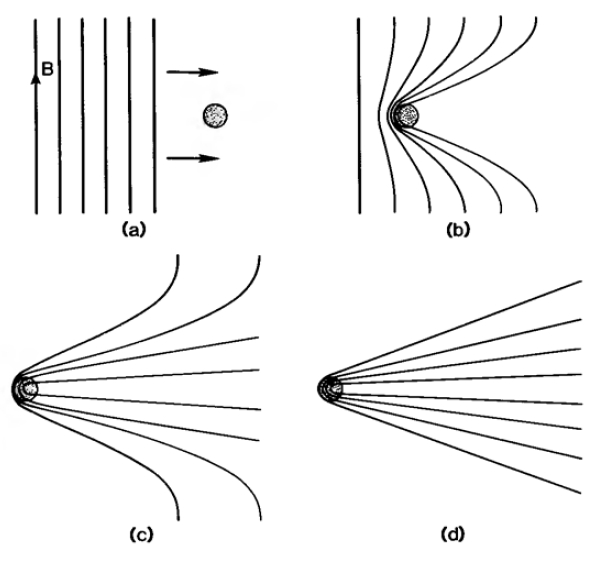
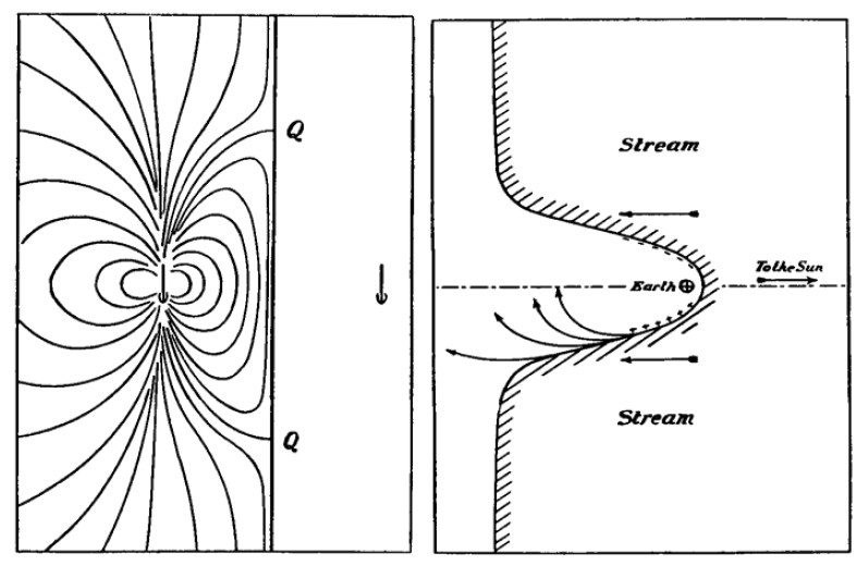
If the auroras were caused by electrons, and if those electrons came from the sun, as was commonly believed among solar-terrestrial researchers in the first half of the twentieth century, then those electrons would have to travel in the company of an equal number of ions, or else the beam would disrupt. That idea can be considered the first model of the streaming ionized plasma of interplanetary space that we call the solar wind. It was an essential element of the geomagnetic-storm model of Chapman and Ferraro, but in their model the solar wind was intermit-tent. It flowed only at active times. However, in 1943, C. Hoffmeister noted that a comet tail was not strictly radial, but lagged behind the comet's radial direction by about 5°. In 1951, L. Biermann correctly interpreted that lag in terms of an interaction between the comet tail and a solar wind. That wind was said to flow at about 450 \(km \cdot s^{-1}\) at all times and in all directions from the sun, although he assumed that the electron density was about 600 cm -3, two orders of magnitude too high. Several years later, in 1957, Hannes Alfven postulated that the solar wind was magnetized and that the solar-wind flow draped that magnetic field over the comet, forming a long magnetic tail downstream in the antisolar direction, as illustrated in Figure 1.11.(A plasma system, or process, is said to be magnetized if its characteristic lengthscale, \(L\), is large compared to the gyroradius.) The cometary ions were confined by that tail in a narrow ribbon between the two tail "lobes." In 1958, E. W. Parker provided the theoretical underpinning for such a flow of magnetized plasma, and in 1962 he showed that in order to be consistent with the geomagnetic records, the electron density of the solar wind should seldom exceed 30 cm 3. Confirmation was not long in coming. That was the dawn of the space age, and soon observations were being returned by both Soviet and American space probes that clearly confirmed the existence of the solar wind and its entrained magnetic field, measured its properties, and demonstrated its pivotalrole in controlling geomagnetic activity and the aurora.