Derivation of KdV Equation in Plasma by Linear Analysis

Introduction

Most interesting problems in continuum mechanics are nonlinear. Plasma problems are perhaps the most nonlinear of all, involving classical mechanics and electromagnetism on an approximately equal footing. This guarantees an abundance of intriguing effects to work on, but also means that solutions are often limited to rather specific situations, involving less generality than modern physicists are trained to expect.

Two of the most important properties characteristic of a plasma are nonlinearity and dispersion. Korteweg de Vries (KdV) equation is a simple model for both of these two phenomena. The KdV equation is given by \[ \frac{\partial U}{\partial \tau} + aU\frac{\partial U}{\partial \xi} + b\frac{\partial^3 U}{\partial \xi^3} = 0 \] where \(\xi\) and \(\tau\) are independent variables and \(a\) and \(b\) are real, nonzero constants. The nonlinear term is convective term \(U\frac{\partial U}{\partial \xi}\) and dispersive term is \(\frac{\partial^3 U}{\partial \xi^3}\) term. It was first derived by Korteweg and de Vries for long surface wave in water. Later, Gardner and Morikawa derived it from a cold-plasma hydromagnetic model describing the long-time behavior of disturbances propagating perpendicular to a magnetic field iwth velocity near the Alfven velocity. Moreover, Washimi and Taniuti have shown that this equation gives a weakly nonlinear description of one-dimensional ion sound wave disturbances traveling near the ion sound speed. In this regard, Su and Gardner have shown that this equation arises in a broad class of weakly nonlinear dispersive systems, just as Burgers' equation arises in a broad class of weakly nonlinear dissipative systems.

Rescale \(\xi\rightarrow\xi b^{1/3}\) and \(U\rightarrow U/ab^{-1/3}\) to give coefficients of unity in front of each term, i.e. \[ \frac{\partial U}{\partial \tau} + U\frac{\partial U}{\partial \xi} + \frac{\partial^3 U}{\partial \xi^3} = 0 \]

Derivation of the KdV equation for nonlinear ion sound waves

Ion sound wave model

We now derive the Korteweg-de Vries equation for the case of ion sound wave disturbances moving with Mach number (defined relative to the ion sound speed) slightly greater than unity in a uniform, magnetic field-free, plasma background. The ions are assumed cold and nondrifting relative to the electrons (\(T_i\ll T_e\)), and a one-dimensional macroscopic description is used. Moreover, electron inertia effects are neglected (\(m_e\rightarrow 0\)) and the isothermal equation of state, \(P_e = n_e k_B T_e\) (\(T_e=const\)), is adopted for the electrons. We then find,

\[ 0 = n_e e \frac{\partial\phi}{\partial x^{'}} - k_BT_e\frac{\partial n_e}{\partial x^{'}} \] which merely describes balance of preesure and electric force. Then we have the Boltzmann relation \(n_e = n_0\exp(e\phi/k_B T_e)\), where \(n_0\) is the uniform background electron density.(Just use the method of separation here). From this equation, we can directly knows number density of electrons by the local electric potential there. The Poisson equation then becomes \[ \partial^2\phi/\partial x^{'2} = 4\pi(e{n_0\exp(e\phi/k_B T_e)-n_i}) \] For the ions, we have \[ \begin{aligned} &\frac{\partial n_i}{\partial t^{'}} + \frac{\partial n_iv_i}{\partial x^{'}} = 0 \\ &\frac{\partial v_i}{\partial t^{'}} + v_i\frac{\partial v_i}{\partial x^{'}} = -\frac{e}{m_i}\frac{\partial\phi}{\partial x^{'}} \end{aligned} \]

Introduce such dimensionless quantities where \[x \equiv \frac{x^{'}}{(k_BT_e/4\pi n_0e^2)^{1/2}} \equiv \frac{x^{'}}{\lambda_D}\] \[ t\equiv t^{'}(\frac{4\pi n_0 e^2}{m_i})^{1/2}\equiv t^{'}\omega_i \] \[ \Phi \equiv \frac{e\phi}{k_BT_e} \] \[ n \equiv n_i/n_0 \] \[ v \equiv \frac{v_i}{(k_BT_e/m_i)^{1/2}}\equiv v_i/v_{th} \]

Then all the above equation can be rewritten as \[ \begin{aligned} &\partial^2\Phi/\partial x^{2} = {\exp(\Phi)-n}\\ &\frac{\partial n}{\partial t} + \frac{\partial nv}{\partial x} = 0 \\ &\frac{\partial v}{\partial t} + v\frac{\partial v}{\partial x} = -\frac{\partial\Phi}{\partial x} \end{aligned} \tag{1} \]

The above equation reproduces the usual ion sound wave dispersion relation \(\omega^2 = (1+(1/k^2))^{-1}\) for perturbations with \(x\) and \(t\) variation of the form \(\exp(i(kx-\omega t))\). It should also be pointed out that a meaningful nonlinear analysis of the above equations must include the effects of charge separation through the term $^2/x{2} $. If we assume charge neutrality, \({n=\exp(\Phi)}\), then we have \[ \frac{\partial v}{\partial t} + v\frac{\partial v}{\partial x} = -\frac{1}{n}\frac{\partial n}{\partial x} \] which is merely momentum equation of ideal gas dynamics. When the spatial gradients become large, however, it is no longer permisible to neglect $^2/x{2} $. It is the dispersive effect of deviations from charge neutrality which eventually limits the buildup of short-wavelength components to the disturbance.

Solitary wave solution

To establish the proper amplitude and variable scaling for deriving the KdV equation, it is useful to first consider the solitary wave solutions associated with the dimensionless equations above. We look for solutions depend on \(x\) and \(t\) through the variable \(x-Mt\) (\(M\) is Mach number \(=V_0/c_s\) = pulse speed / ion-sound-speed). The appropriate boundary conditions for an isolated pulselike solution are \(\Phi\rightarrow 0, v\rightarrow 0, n\rightarrow 0,\Phi^{'}\rightarrow 0, v^{'}\rightarrow 0, n^{'}\rightarrow 0,\) as \(|x-Mt|\rightarrow \infty\), where primes denote differetiation with respect to the variable \(x-Mt\). \(|x-Mt|\rightarrow \infty\) actually means \(x_0 = x-Mt \rightarrow \infty\), which is the boundary at infinitely distance point.

Integrate the continuity and momentum equation above with respect to \(y=x-Mt\), we have, \[ n=M/(M-v) \quad (M-v)^2 = (M^2 - 2\Phi) \] whre the boundary condtion at \(|y|=\infty\) has been enforced. Substitute the above relation into the Poisson equation, multiplying by \(\Phi^{'}\) and integrateing, we find \[ \frac{1}{2}(\Phi^{'})^2 = e^{\Phi} + M(M^2-2\Phi)^{1/2} - (M^2+1) \] where the boundary condition has been enforced also. Now the above equation is a first order nonlinear ODE. The compressive solitary wave solutions to it exist for Mach numbers in the range \(1<M\leq1.6\) with corresponding peak potential \(\Phi_M\) in the range \(0<\Phi_M\leq 1.3\). 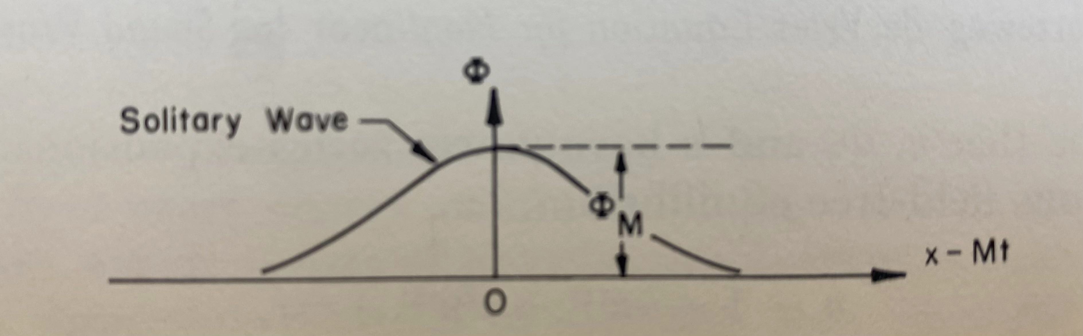For present purposes, we are interested in Mach number slightly greater than unity, \[ 0 < \delta M \equiv M-1 \ll 1 \] which corresponds to a small-amplitude solitary wave with \(\Phi_M\ll 1\). Expanding in \(\Phi\) and \(\delta M\) and retaining leading-order terms, we find, \[ (\Phi^{'})^2 = \frac{2}{3}\Phi^2(3\delta M-\Phi) \] which may be integrated to give \[ \Phi = 3\delta M sech^2((\frac{1}{2}\delta M)^{1/2}(x-Mt)) \] We see from the above equation that the maximum pulse amplitude is \(\Phi_M = 3\delta M\), and that the width of the solitary wave is of order \(\delta M^{-1/2}\).

Here is the Taylor expansion of the hyperbolic function, \[ \begin{aligned} & \sinh x=x+\frac{x^3}{3 !}+\frac{x^5}{5 !}+\frac{x^7}{7 !}+\cdots=\sum_{n=0}^{\infty} \frac{x^{2 n+1}}{(2 n+1) !} \\ & \cosh x=1+\frac{x^2}{2 !}+\frac{x^4}{4 !}+\frac{x^6}{6 !}+\cdots=\sum_{n=0}^{\infty} \frac{x^{2 n}}{(2 n) !} \\ & \tanh x=x-\frac{x^3}{3}+\frac{2 x^5}{15}-\frac{17 x^7}{315}+\cdots=\sum_{n=1}^{\infty} \frac{2^{2 n}\left(2^{2 n}-1\right) B_{2 n} x^{2 n-1}}{(2 n) !},|x|<\frac{\pi}{2} \\ & \operatorname{coth} x=\frac{1}{x}+\frac{x}{3}-\frac{x^3}{45}+\frac{2 x^5}{945}+\cdots=\frac{1}{x}+\sum_{n=1}^{\infty} \frac{2^{2 n} B_{2 n} x^{2 n-1}}{(2 n) !}, 0<|x|<\pi \text { (罗朗级数) } \\ & \operatorname{sech} x=1-\frac{x^2}{2}+\frac{5 x^4}{24}-\frac{61 x^6}{720}+\cdots=\sum_{n=0}^{\infty} \frac{E_{2 n} x^{2 n}}{(2 n) !},|x|<\frac{\pi}{2} \\ & \operatorname{csch} x=\frac{1}{x}-\frac{x}{6}+\frac{7 x^3}{360}-\frac{31 x^5}{15120}+\cdots=\frac{1}{x}+\sum_{n=1}^{\infty} \frac{2\left(1-2^{2 n-1}\right) B_{2 n} x^{2 n-1}}{(2 n) !}, 0<|x|<\pi (罗朗级数) \end{aligned} \]

For \(f(x)=sech(ax)\), the larger \(a\) is, the narrower the pulse is. Introducing \(\epsilon\equiv\delta M\), which is a measure of the pulse amplitude, the argument in the above equation can be expressied as \[ (1/\sqrt{2})(\epsilon^{1/2}(x-t)-\epsilon^{3/2}t) \] This gives the appropriate scaling (in a frame moving with \(M=1\)) of the space and time variables that is required to obtain the KdV equation. It should be kept in mind that the present goal is to construct a weakly nonlinear theory of ion sound waves which describes the evolution of small but finite amplitude disturbances which are traveling near \(M=1\). In order to reconver the solitary wave solution as a special case, which is the minimum demand we make of the theory, the "streched" variables \[\xi = \epsilon^{1/2}(x-t), \quad \tau =\epsilon^{3/2}t\] are introduced in carrying out a nonlinear expansion.

The KdV equation for nonlinear ion sound waves

We assume that \(n,\Phi\) and \(v\) have power series expansions in \(\epsilon\) about a homogeneous field-free equilibrium, i.e., \[ \begin{aligned} &n = 1 + \epsilon n^{(1)} + \epsilon^2 n^{(2)} + \cdots\\ &\Phi = \epsilon \Phi^{(1)} + \epsilon^2 \Phi^{(2)} + \cdots\\ &v = \epsilon v^{(1)} + \epsilon^2 v^{(2)} + \cdots \end{aligned} \]

Furthermore, we transform the \(x\) and \(t\) variables with: \[ \partial/\partial x = \epsilon^{1/2}(\partial/\partial \xi) \quad \partial/\partial t = \epsilon^{3/2}(\partial/\partial \tau) - \epsilon^{1/2}(\partial/\partial \xi) \]

In lowest order, Eqs.(1) become \[ \Phi^{(1)} = n^{(1)},\quad \partial n^{(1)} /\partial \xi = \partial v^{(1)} /\partial \xi, \quad \partial v^{(1)} /\partial \xi = \partial \Phi^{(1)} /\partial \xi \] which gives: \[ \Phi^{(1)} = n^{(1)} = v^{(1)} \] for localized disturbances. To next order in \(\epsilon\), Eqs.(1) become \[ \begin{aligned} &\frac{\partial^2 \Phi^{(1)} }{\partial \xi^2} = \Phi^{(2)} + \frac{(\Phi^{(1)})^2}{2} - n^{(2)}\\ &-\frac{\partial n^{(2)} }{\partial \xi} + \frac{\partial n^{(1)} }{\partial \tau} + \frac{\partial (n^{(1)} v^{(1)})}{\partial \xi} + \frac{\partial v^{(2)} }{\partial \xi} = 0\\ &-\frac{\partial v^{(2)} }{\partial \xi} + \frac{\partial v^{(1)} }{\partial \tau} + v^{(1)}\frac{\partial v^{(1)}}{\partial \xi} =-\frac{\partial \Phi^{(2)} }{\partial \xi} \end{aligned} \] Eliminating \(n^{(2)}\) and \(v^{(2)}\) and making use of result of \(\mathcal{O}(\epsilon)\), we find that \(n^{(1)}\) evolves according to \[ \frac{\partial n^{(1)} }{\partial \tau} + n^{(1)} \frac{\partial n^{(1)}}{\partial \xi} + \frac{1}{2}\frac{\partial^3 n^{(1)}}{\partial \xi^3} = 0 \] which is just the KdV equation with \(a=1, b=1/2\). By virtue of \(\mathcal{O}(\epsilon)\) result, the equations for \(v^{(1)}\) and \(\Phi^{(1)}\) are identiacal to the above equation. It describes the evolution of arbitrary initial disturbances moving near \(M=1\) within the framework of the present macroscopic ion sound wave model. Of course, this equation will be modified if dissipative processes, e.g. Landau damping, play a significant role. Such modification have been considered by Ott and Sudan in relation to the present example, and are summarized later. The origins of the various terms in the above equation are clear. The nonlinear term arises from convection, and the dispersive term arises from deviation from exact charge neutrality.