Local distribution functions
A system is said to be homogeneous (or spatially uniform) when all its local properties are the same at all points in space. In other words, a homogeneous system is invariant under spatial transformations. It is then easily shown that the one-particle distribution function \(f^{\alpha}(\boldsymbol{q},\boldsymbol{v};t)\) must be independent of the \(\boldsymbol{q}\) of the particle in a homogeneous system. They can then always be written in the form
\[ f^{\alpha}(\boldsymbol{q},\boldsymbol{v};t) = n_{\alpha} \phi(\boldsymbol{v};t) \]
where \(n_\alpha=N_\alpha/V\) denotes the constant number density of the particles of species \(\alpha\). \(\phi(\boldsymbol{v};t)\) is the velocity distribution of the particles of the species \(\alpha\) which follows:
\[ \int d \boldsymbol{v}\phi(\boldsymbol{v};t) = 1 \]
If the system is not only homogeneous but also isotropic in velocity space, the velocity distribution function only depends on the magnitude of the vector \(\boldsymbol{v}\):
\[ \phi(\boldsymbol{v};t) = \phi(v;t) \]
Finally, the system is said to be in a stationary state whenever its distribution functions are independent of time.
To each microscopic dynamical function \(b^{\alpha}(\boldsymbol{q},\boldsymbol{v};t)\) corresponds a macroscopic dynamical function \(B(\boldsymbol{x},t)\), obtained by statistical averaging,
\[ B(\boldsymbol{x},t) = \int d \boldsymbol{q} d \boldsymbol{v} b^{\alpha}(\boldsymbol{q},\boldsymbol{v};t) f^{\alpha}(\boldsymbol{q},\boldsymbol{v};t) \]
Usually, such microscopic functions have a common characterisitc structure
\[ b^{\alpha}(\boldsymbol{q},\boldsymbol{v};t) = \beta^{\alpha}(\boldsymbol{v}) \delta(\boldsymbol{q} - \boldsymbol{x}) \]
Actually this looks like a coordinate transformation from microscopic particle coordinate to macroscopic Euler coordinate.
Therefore, we have \[ B(\boldsymbol{x},t) = \int d \boldsymbol{q} d \boldsymbol{v} \beta^{\alpha}(\boldsymbol{v}) \delta(\boldsymbol{q} - \boldsymbol{x}) f^{\alpha}(\boldsymbol{q},\boldsymbol{v};t) \]
Denote local velocity distribution function,
\[ f^{\alpha}(\boldsymbol{v};\boldsymbol{x},t) = \int d \boldsymbol{q}\delta(\boldsymbol{q} - \boldsymbol{x})f^{\alpha}(\boldsymbol{q},\boldsymbol{v};t) \]
Then we have \[ B(\boldsymbol{x},t) = \int d \boldsymbol{v} \beta^{\alpha}(\boldsymbol{v}) f^{\alpha}(\boldsymbol{v};\boldsymbol{x},t) \]
It may be said that \(f^{\alpha}(\boldsymbol{v};\boldsymbol{x},t)\) is a functional field: to each point in space and to each time it assigns a function of \(\boldsymbol{v}\). Although the difference between ordinary and localized distribution functions may seem trivial in this case, it is worth insisting on their difference nature.
Macroscopic quantities
Whenever the dynamical function \(\beta{(\boldsymbol{v})}\) is a ploynomial in the three components of the velocity, i.e
\[ \beta{(\boldsymbol{v})} = \sum_{r_1=0}^{s_1}\sum_{r_2=0}^{s_2}\sum_{r_3=0}^{s_3} a_{r_1r_2r_3}v_x^{r_1}v_y^{r_2}v_z^{r_3} \] the corresponding average will be called a moment (of order \(s=s_1+s_2+s_3\)) of the local distribution function.
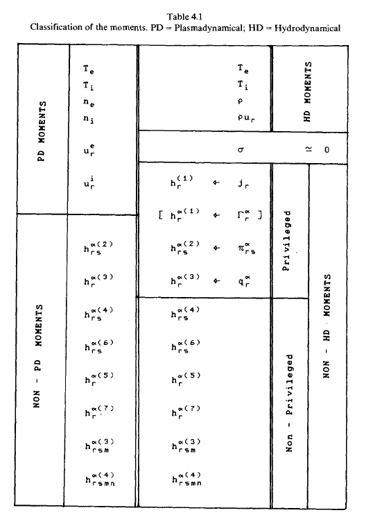
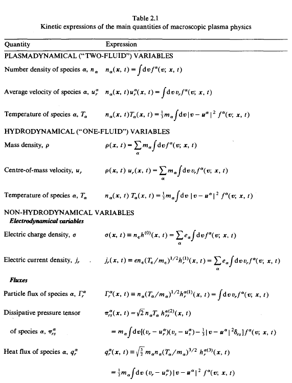
Here we give all relations between microscopic and macroscopic quantities in a table.
Some time scale of kinetic equation
In order to construct the transport theory, i.e. in order to obtain closed hydrodynamical and electrodynamical equations, we need to solve the kinetic equation to get high order moments. Because of its complexity, an exact solution is practically impossible; therefore, we need approximation methods, valid in various conceivable regimes. A clue as to the choice of approximation methods is provided by an analysis of the various characteristic times involved in the kinetic equation. By a trivial dimensional argument, each term on the R.H.S of the kinetic equation must have a dimension \(f^\alpha/T\), where \(T\) is some characteristic time, but the time is different for each term.
The free flow term introduces a characteristic time \(\tau_H^\alpha\) which may be called the hydrodynamical time. It is related to the spatial variation of the local distribution function. It is can be estimated as
\[ \frac{1}{\tau_H^\alpha} \sim \frac{V_{\tau_\alpha}}{L_H} \]
where \(V_{\tau_\alpha}\) is the thermal velocity of species \(\alpha\)(the reason to choose thermal velocity as characteristic velocity is because \(v\) in kinetic equation stands for velocity of moleculars, which has characterist velocity as thermal velocity), and \(L_H\) is the length of the gradient of the density, the velocity or the temperature, whichever is shorter:
\[ \frac{1}{L_H} = max(\frac{|\nabla A(x)|}{|A(x)|}) \]
In most situations of interest, the gradients are due to some experimental preparation obtained by a macroscopic device, such that the length of the gradients is very large compared to molecular dimensions. It follows that \(\tau_H^\alpha\) can be considered as a very long time, and therefore the characteristic variations related to the free-flow term are slow.
However, the Vlasov term of the kinetic equation poses some complicated problems. In the first place, there may be external high-frequency fields present (such as those produced by a laser, or by an RF source used for heating a tokamak, etc). Such fields will induce fast motions of the electrons. But even in the absence of external fields, there is a possibility of fast internal motions. Indeed, any fluctuations producing a local charge separation leads to a force on the electrons. The latter start oscillating with the well-knowing plasma frequency \(\omega_{pe}\), which is in general a high frequency wave. The problem of the coupling of the fast (electrodynamic) motions with the slow (hydrodynamic) motions is a quite interesting, but rather difficult problem. Here, we first consider slowly varying electromagnetic fields: the influence of high-frequency phenomena is left for later discussion. So here, we also assume that \(L_H, \tau_H\) are also the characteristic length and time scales of the electric field \(\boldsymbol{E}\) and of the magnetic field \(\boldsymbol{B}\).
This approximation may seem incorrect because of the existence, even in the absence of the external high-frequency fields. However, in a linear theory, these effects do not influence the slow plasma motions in which we are interested here. This can be understood from the following schematic argument.
All the hydrodynamic quantities as well as the electromagnetic fields may be split into a slow varying part \(A_s\) and a rapidly varying part \(A_f\): \(A = A_s + A_f\) (imagine it can be decomposed to a slow varying wave and a fast varying wave). There equation of evolution can be written as
\[ \partial_t A_s = \Phi_s(A_s, A_f) \quad \partial_t A_f = \Phi_f(A_s, A_f) \]
\(\Phi(A)\) represents some, generally non-linear, combinations of both the slow and fast part and of their gradients. If these equations are linearized as in classical transport theory, it is clear that the slow(fast) variables can only be determined by the slow(fast) variables in the R.H.S.(ignore the nonlinear interaction between slow and fast part.) The evolution of the slow variables can then be studied independently of the fast ones, as will indeed be done here. If however, non-linear effects become important (e.g. when the amplitude of the fast electromagnetic fields is high, as for instance in the presence of an intense laser beam or of an intense RF heating beam in a tokamak), two high-frequency components may couple and produce a low-frequency beat-wave, which influences the slow motions. This type of nonlinear coupling will be studied later.(This is an another excellent example illustrating the meaning of linear and non-linear).
If the main assumption is accepted, the well-known pre-Maxwell approximation follow very easily. Indeed, the Maxwell equation leads to the following estimate of the ratio of the electric and magnetic fields:
\[ \frac{|E|}{L_H} \approx \frac{1}{c}\frac{|B|}{\tau_H} \]
On the other hand,
\[ \frac{|B|}{L_H} \approx \frac{1}{c}\frac{|E|}{\tau_H} + \frac{4\pi}{c}j \]
Combining these two equations, we find that the displacement current term is of order \(L_H^2/\tau_H^2c^2\) compared to the L.H.S. As \(L_H/\tau_H\) is of the order of the hydrodynamic velocity, we may conclude
\[ |\frac{1}{c}\partial_t E| \approx \frac{u^2}{c^2} |\nabla\times B| \]
Hence, whenever the motion of the plasma is non-relativisitic, the displacement current can be neglected and the slow varying field obey the pre-Maxwell equation. In this form, take divergence at Amphere's Law, the current density obeys the constraint:
\[ \nabla\cdot\boldsymbol{J} \approx 0 \]
But the charge balance is valid whatever condition.In order to ensure the mutual compatibility of these conditions, we necessarily must have
\[ \partial_t \sigma \approx 0 \]
However, the above equaton should not be considered as an exact equation; it only means that the charge density is a slowly varying function. As for the size of this quantity, it may be estimated from the following argument. It is well known that a plasma cannot support large local charge separations. It is therefore almost always true that, in all points \(x\) and at all times \(t\),
\[ |n_e(x,t) - n_i(x,t)| \ll \frac{1}{2} (n_e(x,t) + n_i(x,t)) \]
This will be called the local quasi-neutrality condition. It implies,
\[ \sigma(x,t) \ll \frac{e}{m_e}\rho_e(x,t) = en_e(x,t) \] \[ \sigma(x,t) \ll \frac{Ze}{m_i}\rho_i(x,t) = en_i(x,t) \]
As a result, the charge density can be neglected in all the hydrodynamical equations, except for the term \(\sigma\boldsymbol{E}\) in momentum equation. This term is, however, negligible for a different reason. A similar dimensional argument leads to the estimate:
\[ \frac{\sigma E}{c^{-1}|J\times B|} \approx \frac{(\nabla\cdot E)E}{(\nabla\times B)B} \approx \frac{L_H^{-1}E^2}{L_H^{-1}B^2} \approx \frac{u^2}{c^2} \]
So in non-relativisitc regime, the contribution from electric force is negligible. The only place where \(\sigma\) cannot be neglected is the Poisson equation. This equation, however, acquires a different status. Indeed, the generalized Ohm law can be used for completely determining the electric field. Hence the Poisson equation becomes superfluous: it only serves for defining the charge density - a quantity which does not influence the motion of the plasma in the present approximation.
From the above analysis, we can also see that if the flow moves fast enough comparable to the speed of light, then the influence of electric charge and field cannot be ignored anymore. The system is not locally neutral as in non-relativisitc case.
Finally, the time scale for last collision term is called relaxation time \(\tau_\alpha\). The relaxation time is an internal, molecular parameter, whose values depends on the state of the plasma (density and temperature).
Once we separate different scale, we can discuss different scales separately. It is similiar to make nonlinear problem becomes a linear problem. Here, we have already get a physical picture as follows. Starting from an arbitrary initial state, the collisions would tend - if they were alone - to bring the system very quickly to a stationary state: the thermal equilibrium. But the slow processes - free flow and electromagnetic processes - prevent the plasma from reaching this state. The result is that, after a short time, of the order of the relaxation time \(\tau_\alpha\), the plasma reaches a state very close to the equilibrium. From here on, the distribution funcitons evolve on the slow time scale.
In plasma, collision frequencies between species and within species are quite different. Collisions between particles of equal mass are quite effective in redistributing momentum and energy among the partners, collisions between unlike particles of largely different mass behave very poorly from this point of view. As a result, the relaxtion towards the equilibrium proceeds in two stages. First, the like particle collisions bring each component to its own state of local equilibrium. Afterwards, the temperature and average velocities tend to equilibrate, but this process is much slower, especially for the temperatures: the time scale involved is of the same order as the slow time scales related to the free-flow and the electromagnetic processes. Thus, in a sense, the unlike-particle collisions must be treated on the sam footing as the slow processes.
The Hermitian moment expansion
In collision dominated plasma, after a short transition time, the state of plasma remains close to the local plasma equilibrium. For this reason, the local plasma equilibrium will be called a reference state. The distribution functions can then conveniently be written in the form
\[ f^\alpha(\boldsymbol{v};\boldsymbol{x},t) = f^{\alpha 0}(\boldsymbol{v};\boldsymbol{x},t)[1 + \hat\chi^\alpha(\boldsymbol{v};\boldsymbol{x},t) ] \]
The functions \(\hat\chi^\alpha(\boldsymbol{v};\boldsymbol{x},t)\) measure the deviation of the local distribution function \(f^\alpha\) from the reference state. It is clear that the whole information about the real state of the plasma is contained in \(\hat\chi^\alpha(\boldsymbol{v};\boldsymbol{x},t)\).
We now introduce a condition which is very useful in providing an unambiguous interpretation of the results. Here we construct the above representation in such a way that the parameters \(n_\alpha,u_r^\alpha,T_\alpha\) entering the definition of the reference state do coincide with the exact value of the density, velocity and teperature of each species. (It means that the \(n_\alpha,u_r^\alpha,T_\alpha\) in reference state is just the macroscopic quantities, although I think it should be so hhh). Then we can have constraints on the deviations:
\[ \int d \boldsymbol{v} f^{\alpha0}\hat\chi^\alpha = 0 \quad \int d \boldsymbol{v} f^{\alpha0}v_r\hat\chi^\alpha = 0 \quad \int d \boldsymbol{v} f^{\alpha0}v^2\hat\chi^\alpha = 0 \]
Before continuing, it is convenient to note that the distribution functions \(f^{\alpha 0}\) depend on the velocity \(v\) only through the dimensionless variable \[ \boldsymbol{c}=\left(\frac{m_\alpha}{T_\alpha(\boldsymbol{x}, t)}\right)^{1 / 2}\left[\boldsymbol{v}-\boldsymbol{u}^\alpha(\boldsymbol{x}, t)\right] . \] As most of the important quantities are averages of powers of the relative velocities \(\boldsymbol{v}-\boldsymbol{u}^\alpha\), it is clear that \(\boldsymbol{c}\) is a quite convenient variable. We shall therefore express all functions in terms of it. Clearly, some care must be taken by noting that the passage from \(v\) to \(c\) is different for the electrons and for the ions, and that the coefficients of the transformation depend on \(x\) and \(t\). We now write the local plasma equilibrium distribution as \[ f^{\alpha 0}(\boldsymbol{v} ; \boldsymbol{x}, t)=n_\alpha(\boldsymbol{x}, t)\left(\frac{m_\alpha}{T_\alpha(\boldsymbol{x}, t)}\right)^{3 / 2} \phi^{\alpha 0}(\boldsymbol{c} ; \boldsymbol{x}, t), \] where \[ \phi^{\alpha 0}(c ; x, t) \equiv \phi^0(c)=(2 \pi)^{-3 / 2} \exp \left(-c^2\right) \]
We note the very important fact that the reference state \(\phi^{\alpha 0}\), when expressed in terms of the variables \(c\), is a stationary, homogeneous and isotropic state, whereas considered as a function of the original variable \(v\), it has none of these properties. Moreover, \(\phi^{\alpha 0}(c)\) is the same function for the electrons and for the ions, it is therefore independent of the superscript \(\alpha\). The dimensionless reference distribution function is normalized as \[ \int \mathrm{d} c \phi^0(c)=1 \] We now express the complete distribution functions as \[ \begin{aligned} f^\alpha(\boldsymbol{v} ; \boldsymbol{x}, t) & =n_\alpha(\boldsymbol{x}, t)\left(\frac{m_\alpha}{T_\alpha(\boldsymbol{x}, t)}\right)^{3 / 2} \phi^\alpha(\boldsymbol{c} ; \boldsymbol{x}, t) \\ & =n_\alpha(\boldsymbol{x}, t)\left(\frac{m_\alpha}{T_\alpha(\boldsymbol{x}, t)}\right)^{3 / 2} \phi^0(c)\left[1+\chi^\alpha(c ; \boldsymbol{x}, t)\right] . \end{aligned} \] The constraints, expressed in the new variables, are \[ \int \mathrm{d} c \phi^0 \chi^\alpha=0, \quad \int \mathrm{d} c \phi^0 c_r \chi^\alpha=0, \quad \int \mathrm{d} c \phi^0 c^2 \chi^\alpha=0 . \] We now start the investigation of our main problem, which consists of finding an approximate solution for the unknown functions \(\chi^\alpha\). (It is different from methods from textbook like global expansion with a small parameter \(\epsilon\), it just directly let you to find a new function, it is harder I think.) Several methods have been developed for this purpose. The most ancient and celebrated one is the Chapman-Enskog method, developed independently by these authors already in 1916 (Chapman and Cowling 1952). Grad's (1949) moment method has also been widely used. Finally, Résibois's (1970) more recent projection operator method is quite elegant and useful in the linear domain. All these methods, in various versions, have been applied to the problem of transport in plasmas. Here, we start directly with a method which has - in our opinion - the advantage of clarity and simplicity. It is close in spirit to Grad's method but has features in common with the two others as well.
The general idea is quite straightforward. Adopting a technique widely used in quantum mechanics, we start by expanding the unknown functions \(\chi^\alpha\) in a series of orthogonal polynomials. The determination of the coefficients of this series is equivalent to the determination of \(\chi^\alpha\). The kinetic equation provides an infinite set of equations for these coefficients. If we are clever (lucky?) the series will rapidly converge. A truncated set of equations will then be sufficient for the determination of the transport properties with the required precision. The first step consists of choosing an adequate set of orthogonal polynomials. We want an expansion of \(\chi^\alpha(\boldsymbol{c} ; \boldsymbol{x}, t)\), considered as a function of \(\boldsymbol{c}\), i.e. o the three scalar variables \(c_x, c_y, c_z\). As the local equilibrium distribution obviously plays a crucial role in the theory, a very natural basis is provided by the Hermite polynomials, which are orthogonal with respect to a Gaussian weight function(Since reference state also has exponetial function, it is natrual to let \(\chi\) also has such form, it is a guess).
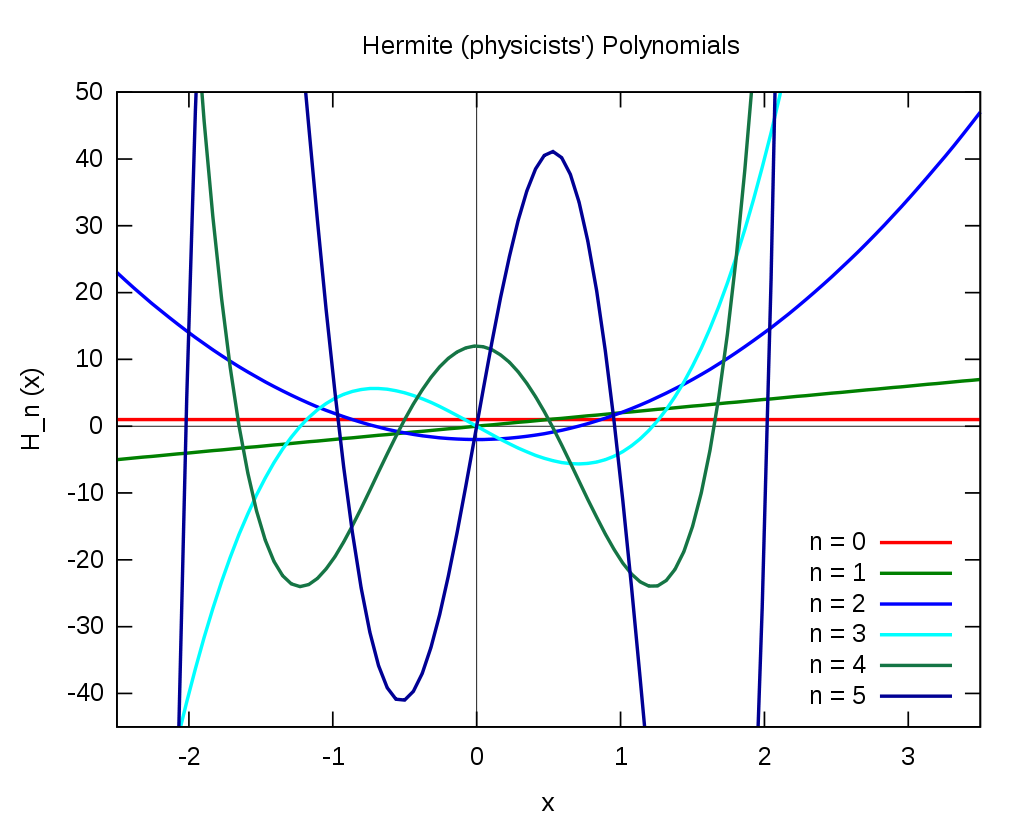
The Hermite polynomials are given by
\[ H_n(x)=(-1)^n e^{x^2} \frac{d^n}{d x^n} e^{-x^2} \]
The first eleven physicist's Hermite polynomials are: \[ \begin{aligned} H_0(x) & =1 \\ H_1(x) & =2 x \\ H_2(x) & =4 x^2-2 \\ H_3(x) & =8 x^3-12 x \\ H_4(x) & =16 x^4-48 x^2+12 \\ H_5(x) & =32 x^5-160 x^3+120 x \\ H_6(x) & =64 x^6-480 x^4+720 x^2-120 \\ H_7(x) & =128 x^7-1344 x^5+3360 x^3-1680 x \\ H_8(x) & =256 x^8-3584 x^6+13440 x^4-13440 x^2+1680 \\ H_9(x) & =512 x^9-9216 x^7+48384 x^5-80640 x^3+30240 x \\ H_{10}(x) & =1024 x^{10}-23040 x^8+161280 x^6-403200 x^4+302400 x^2 - 30240 \end{aligned} \]
The picture is:
As we are considering here functions of three variables, we need to use the so-called tensorial Hermite polynomials, a generalization of the well-known one-dimensional Hermite polynomials. But even at this level, we still have a choice. It is found tha the use of the straightforward three-dimensional generalization of the Hermite polynomials ("reducible tensorial Hermite polynomials") (as was done by Grad 1949) leads to a rather untransparent expansion.
It turns out that a representation in which the various types of anisotropy of the distribution function are clearly exhibited, is the most convenient guide for reasonable truncation approximations. Such a representation would be of the form \[ \begin{aligned} \chi^\alpha(\boldsymbol{c} ; \boldsymbol{x}, t)= & A^\alpha(c ; \boldsymbol{x}, t)+c_r B_r^\alpha(c ; \boldsymbol{x}, t) \\ & +\left(c_r c_s-\frac{1}{3} c^2 \delta_{r s}\right) C_{r s}^\alpha(c ; \boldsymbol{x}, t)+\cdots, \end{aligned} \] where \(A^\alpha\) is a scalar function, \(B_r^\alpha\) a vector function, \(C_{r s}^\alpha\) a symmetric traceless tensor function, etc. All of these depend only on the absolute value of the variable \(\boldsymbol{c}\), as well as on the variables \(\boldsymbol{x}\) and \(t\). These functions are sometimes called "anisotropies" of successive orders. The above wepresentation is taken as a basic Ansatz in the Chapman-Enskog method (Chapman and Cowling 1952, Braginskii 1965, Ferziger and Kaper 1972). In that method, the functions \(A^\alpha\), \(B_r^\alpha, C_{r s}^\alpha\) are then further expanded in series of Laguerre-Sonine polynomials of the single variable \(c\), and each of them is truncated at some appropriate level. (The CE expansion is more complicated for full Boltzmann equation than BGK approximation).
The reason for the usefulness of such a representation is clear. Our main use of the functions \(\chi^\alpha\) will be in the calculation of the relevant fluxes appearing in the hydrodynamical balance equations, such as the heat flux \(q_r^\alpha\) and the pressure tensor \(\pi_{r s}^\alpha\). In a linear theory (no interaction between vector and tensor part), the former will be entirely determined by the vector part of \(\chi^\alpha\), i.e. by \(B_r^\alpha\), whereas the pressure tensor involves only the tensor part of \(\chi^\alpha\). Even in a non-linear theory, the explicit exhibition of the anisotropies helps considerably in the calculations.
It is found that the most convenient expansion, which exhibits explicitly the anisotropies, is obtained by using the irreducible tensorial Hermite polynomials, \(H_{r_1 \ldots r_s}^{(m)}(c)\), \[ \begin{aligned} \chi^\alpha(c ; x, t)= & \sum_{n=0}^{\infty} h^{\alpha(2 n)}(x, t) H^{(2 n)}(c) \\ & +\sum_{n=0}^{\infty} h_r^{\alpha(2 n+1)}(x, t) H_r^{(2 n+1)}(c) \\ & +\sum_{n=1}^{\infty} h_{t s}^{\alpha(2 n)}(x, t) H_{r s}^{(2 n)}(c)+\cdots \end{aligned} \] The function \(\chi^\alpha(c)\) of the continuous vector variable \(c\) is thus represented by a denumerable infinite set of coefficients \(h^{\alpha(m)}\) called the (irreducible) Hermitian moments of the distribution function; these, in turn, are classified as scalar Hermitian moments \(h^{\alpha(2 n)}\), vector Hermitian moments \(h_r^{\alpha(2 n+1)}\), traceless tensor Hermitian moments \(h_{r s}^{\alpha(2 n)}\), etc. The moments are related to the original function as \[ h_{r_1 \ldots r_q}^{\alpha(m)}(x, t)=\int \mathrm{d} c \phi^0(c) H_{r_1 \ldots r_q}^{(m)}(c) \chi^\alpha(c ; x, t) \] Alternatively, the moment \(h_{r_1 \ldots r_q}^{\alpha(m)}\) (for \(m \neq 0\) ) can also be interpreted as the average value of the Hermite polynomial \(H_{r_1 \ldots r_q}^{(m)}(c)\), calculated with the full (dimensionless) distribution function \(\phi^\alpha(\boldsymbol{c} ; \boldsymbol{x}, t)\), eq. (3.8), \[ h_{r_1 \ldots r_q}^{\alpha(m)}(x, t)=\int \mathrm{d} c \phi^0(c)\left[1+\chi^\alpha(c ; x, t)\right] H_{r_1 \ldots r_q}^{(m)}(c), \quad m \neq 0 . \] Indeed, the orthogonality of any polynomial \(H_{\ldots}^{(m)}\) to \(H^{(0)} \equiv 1\) implies \[ (2 \pi)^{-3 / 2} \int \mathrm{d} c \exp \left(-\frac{1}{2} c^2\right) H_{r_1 \cdots r_q}^{(m)}(c)=\delta_{m, 0} . \] Hence, in the local equilibrium state, the average value of all Hermite polynomials of non-zero degree is identically zero.
It is seen that the tensorial polynomials are of the form \[ \begin{aligned} & H_r^{(2 n+1)}(c)=c_r f^{(2 n+1)}(c), \\ & H_{r s}^{(2 n)}(c)=\left(c_r c_s-\frac{1}{3} c^2 \delta_{r s}\right) g^{(2 n)}(c), \end{aligned} \] where \(f^{(2 n+1)}(c), g^{(2 n)}(c)\) are functions of the absolute value of the vector \(c\).
Next, we must be sure that the constraints are satisfied. Because of the orthogonality of the Hermite polynomials, the constraints take a very simple form. They amount to requiring that three Hermitian moments by identically zero for every acceptable deviation \(\chi^\alpha\) : \[ h^{\alpha(0)} \equiv 0(density), \quad h^{\alpha(2)} \equiv 0(energy), \quad h_r^{\alpha(1)} \equiv 0 (momentum). \] Finally, we note that the moments \(h_{r s}^{\alpha(2)}\)(stress tensor) and \(h_r^{\alpha(3)}\)(heat flux) have a very important physical meaning. Using table 3.2.1, we have \[ \begin{aligned} \pi_{r s}^\alpha & =m_\alpha \int \mathrm{d} v\left[\left(v_r-u_r^\alpha\right)\left(v_s-u_s^\alpha\right)-\frac{1}{3}\left|v-\boldsymbol{u}^\alpha\right|{ }^2 \delta_{r s}\right] f^\alpha \\ & =m_\alpha \frac{T_\alpha}{m_\alpha} n_\alpha \int \mathrm{d} c\left[c_r c_s-\frac{1}{3} c^2 \delta_{r s}\right] \phi^0\left[1+\chi^\alpha\right] \\ & =T_\alpha n_\alpha \sqrt{2} \int \mathrm{d} c H_{r s}^{(2)} \phi^0 \chi^\alpha . \end{aligned} \] Hence, we find a very simple relation between the pressure tensor and the second-order tensor Hermitian moment: \[ \pi_{r s}^\alpha=\sqrt{2} n_\alpha T_\alpha h_{r s}^{\alpha(2)} . \] We easily derive a similar relation between the heat flux and the third-order vector Hermitian moment: \[ q_r^\alpha=\sqrt{\frac{5}{2}} m_\alpha\left(\frac{T_\alpha}{m_\alpha}\right)^{3 / 2} n_\alpha h_r^{\alpha(3)} \]
We have now achieved the desired series expansion, exhibiting the tensorial symmetries explicitly. For calculational purposes, these series must be truncated. This truncation process is done in two stages. As said before, in a linear theory we shall only need the vector and traceless second-rank tensor parts (no higher order tensor). In particular, it is found that the scalars and the anisotropies of order three and higher give rigorously no contribution to the entropy production (in the linear regime). We thus neglect all other anisotropies and write \[ \chi^\alpha(\boldsymbol{c} ; \boldsymbol{x}, t) \approx c_r B_r^\alpha(c ; \boldsymbol{x}, t)+\left(c_r c_s-\frac{1}{3} c^2 \delta_{r s}\right) C_{r s}^\alpha(c ; \boldsymbol{x}, t) . \] The series for \(B_r^\alpha\) and \(C_{r s}^\alpha\) can then be truncated at various levels. We consider here three successive approximations. (A) The thirteen moment \((13 \mathrm{M})\) approximation *: \[ \begin{aligned} & c_r B_r^\alpha(c ; \boldsymbol{x}, t)=h_r^{\alpha(3)}(\boldsymbol{x}, t) H_r^{(3)}(\boldsymbol{c}), \\ & \left(c_r c_s-\frac{1}{3} c^2 \delta_{r s}\right) C_{r s}^\alpha(c ; \boldsymbol{x}, t)=h_{r s}^{\alpha(2)}(\boldsymbol{x}, t) H_{r s}^{(2)}(\boldsymbol{c}) . \end{aligned} \] (B) The twenty-one moment (21 M) approximation: \[ \begin{aligned} & c_r B_r^\alpha(c ; x, t)=h_r^{\alpha(3)}(x, t) H_r^{(3)}(c)+h_r^{\alpha(5)}(x, t) H_r^{(5)}(c), \\ & \left(c_r c_s-\frac{1}{3} c^2 \delta_{r s}\right) C_{r s}^\alpha(\boldsymbol{c} ; \boldsymbol{x}, t)=h_{r s}^{\alpha(2)}(\boldsymbol{x}, t) H_{r s}^{(2)}(\boldsymbol{c})+h_{r s}^{\alpha(4)}(\boldsymbol{x}, t) H_{r s}^{(4)}(\boldsymbol{c}) . \end{aligned} \] (C) The twenty-nine moment (29 M) approximation: \[ \begin{aligned} & c_r B_r^\alpha(c ; x, t)=h_r^{\alpha(3)}(x, t) H_r^{(3)}(\boldsymbol{c})+h_r^{\alpha(5)}(\boldsymbol{x}, t) H_r^{(5)}(c) \\ & \quad+h_r^{\alpha(7)}(\boldsymbol{x}, t) H_r^{(7)}(c), \\ & \left(c_r c_s-\frac{1}{3} c^2 \delta_{r s}\right) C_{r s}^\alpha(\boldsymbol{c} ; \boldsymbol{x}, t) \\ & =h_{r s}^{\alpha(2)}(\boldsymbol{x}, t) H_{r s}^{(2)}(\boldsymbol{c})+h_{r s}^{\alpha(4)}(\boldsymbol{x}, t) H_{r s}^{(4)}(\boldsymbol{c})+h_{r s}^{\alpha(6)}(\boldsymbol{x}, t) H_{r s}^{(6)}(\boldsymbol{c}) . \end{aligned} \]
This is just like what we've done in small parameter expansion, but here the latter term means high frequency (maybe?) but not higher derivative (maybe there is connection, after all they are all high order quantities.)
So now, we have gone through the whole process of the Hermite expansion. Compared to order balance in classical perturbation methods, here we directly choose a base to represent the analytical form of the perturbation function. Then the convergence relies on whether the basis are enough to fit the unknown function (but I haven't learned about how to analyze such approximation methods, it is something more like numerical methods.) Beside, here, tensorial Hermite polynomials are employed, which can express anisotropy more natrually. Therefore, here we have two types of truncation. The first type is choosing the order of tensor, it is found that second order is enough. The second type is truncation of basis. It is just like choose Fourier mode. Here, three successful approximation are introduced, i.e. 13M, 21M and 29M, among which 21M behaves best.
The thirteen moment (13M) approximation just keeps the five plasmadynamical moments \(n_\alpha, \mathbf{u}_\alpha, T_\alpha\), the three components of the heat flow vector \(\mathbf{h}_\alpha\), and the five independent components of the anisotropic pressure tensor \(\pi_\alpha\). The \(21 \mathrm{M}\) approximation adds the three components of the fifth order Hermitian moment \(\overline{\mathbf{h}}_\alpha^{(5)}\) and the five components of the fourth order Hermitian moment \(\overline{\mathbf{h}}_\alpha^{(4)}\), etc. Balescu demonstrates that the classical transport coefficients in the \(21 \mathrm{M}\) approximation agree to within \(1 \%\) with the ones obtained much earlier by Braginskii by a very different representation, but it deviates in some important aspects of the interpretation.
Next, we have to find the exact value of various moments, some of them are related to equilibrium distribution function, some of them are related to perturbation function. We need to construct a set of equations to solve all these moments, which is the so-called Moments Methods. In hydrodynamical regime, they are also called fluid equation. Various moments need to be solved are listed as follows: